どうも、Beyond the Pixelです。心臓のCT画像は、心臓の形態を非侵襲的に評価する上で不可欠なツールであり、心筋壁厚は肥大型心筋症の診断、突然心臓死のリスク層別化、心不全における心室リモデリングの追跡など、重要な臨床的指標となります。これらの測定値を確実に得るためには、心臓の正確な三次元(3D)幾何学的形状が不可欠です。しかし、臨床の心臓CTでは、スライス間の間隔が粗いことが一般的です。このため、二次元(2D)のセグメンテーション(画像から特定の領域を識別する処理)マスクを重ね合わせて3D形状を形成すると、表面がギザギザとした階段状になり、臨床医が必要とする壁厚測定の精度を著しく低下させてしまいます。
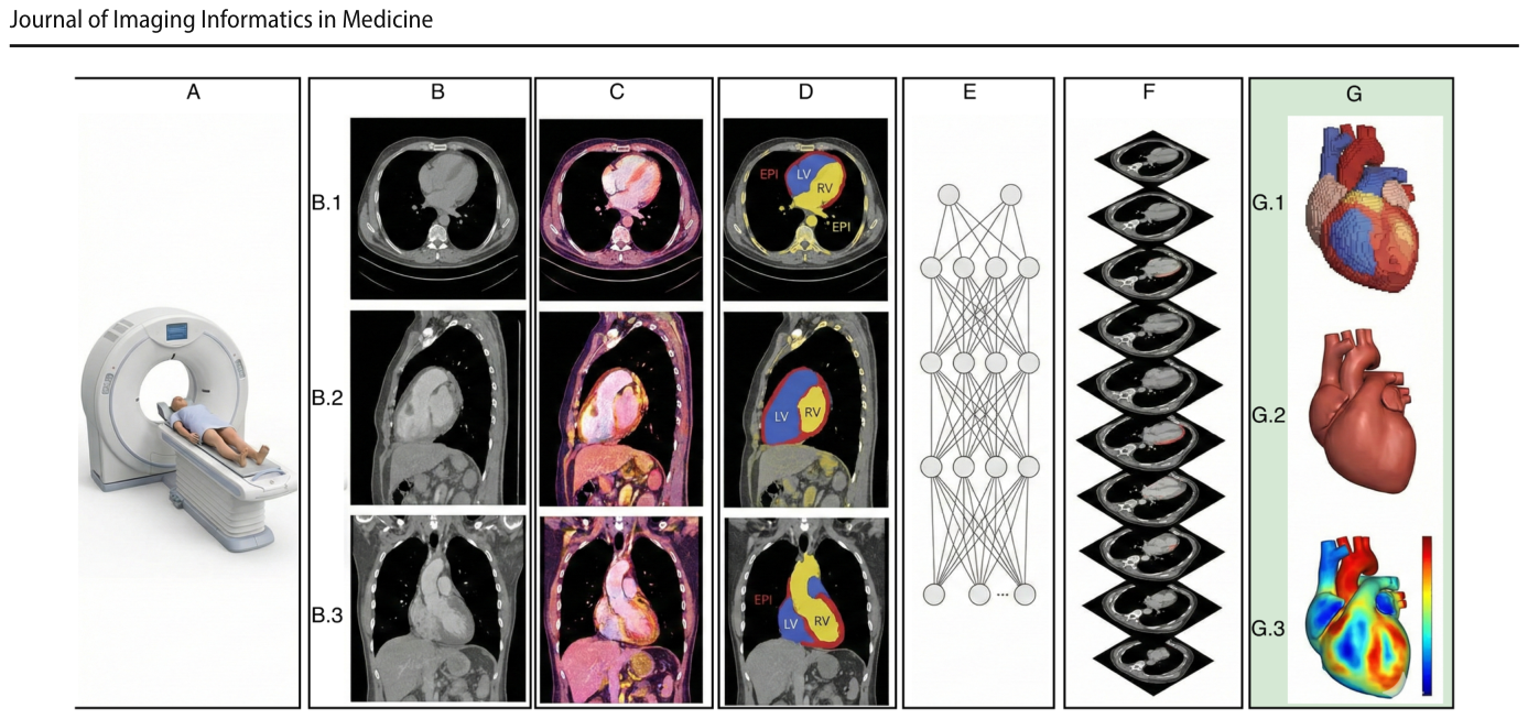
Figure 1. Fig. 1 A patient undergoing cardiac CT (A) generates a volumet- ric dataset that clinicians inspect across axial (B.1), sagittal (B.2), and coronal (B.3) planes (B). After preprocessing (C), an automated segmentation network (D, E) delineates cardiac structures slice by slice. The predicted masks are stacked (F) to form an initial 3D解説: 心臓CT検査の対象者(A)が、臨床医が軸位(B.1)、矢状位(B.2)、冠状位(B.3)で検査する体積データセットを生成する(B)。前処理(C)後、自動セグメンテーションネットワーク(D, E)がCTスライスから心臓構造を輪郭化する。予測されたマスクは重ね合わされて(F)初期の3D表現を形成するが、CTの異方性な間隔により著しい階段状のアーティファクトが発生する(G.1)。本研究の間隔認識型再構築(G.2)は、滑らかで解剖学的に忠実な表面を生成し、そこから壁厚を測定し臨床基準(G.3)に対して検証できる(G)。
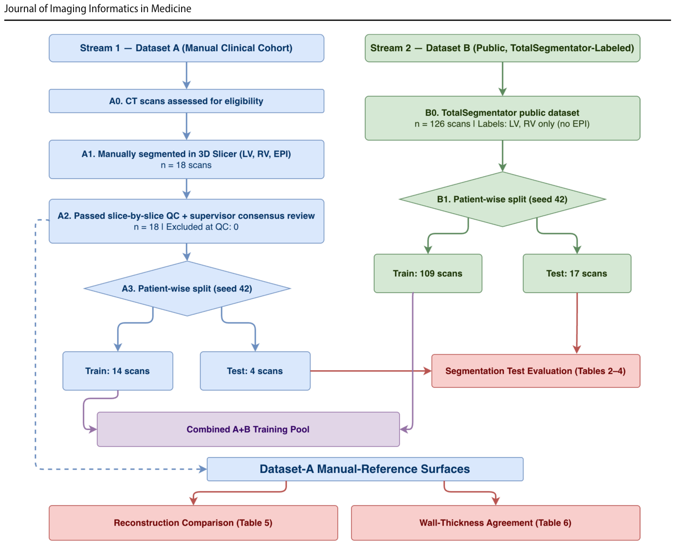
Figure 2. Fig. 2 STARD-style subject and data flow for this methodological agreement study (not a diagnostic-accuracy trial). Two intake streams are shown: Dataset A (manual clinical cohort) is segmented, quality- controlled, and split subject-wise into 14 training and 4 held-out test scan volumes; Dataset B (public, TotalSegmentator-labeled, LV/RV only) is split into 109 training and 17 test scans. The combined pool解説: この方法論的合意研究のSTARD形式の対象者およびデータフローが示されています。2つのデータ取り込みストリーム(データセットA:手動臨床コホート、データセットB:公開、TotalSegmentatorラベル付け、LV/RVのみ)があり、それぞれがセグメンテーション、品質管理、対象者ごとの分割を経て、トレーニング用とテスト用に分けられます。データセットAの手動参照表面は、メッシュレベルの再構築評価と壁厚評価に用いられます。
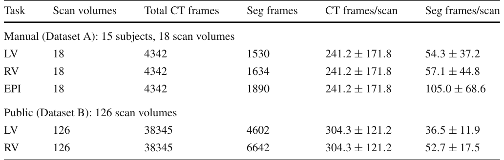
Table 1. Table 1 Dataset summary and annotation density for LV, RV, and EPI. Dataset A comprises 15 unique subjects contributing 18 scan volumes, because 3 subjects were imaged both before and after intervention. Counts below are per scan volume, and per-scan statistics are mean ± SD across the 18 scan volumes. Dataset B contributes 126 scan volumes解説: LV、RV、EPIのデータセット概要とアノテーション密度を示しています。データセットAは15名の固有の対象者からなる18のスキャンボリュームで構成され、データセットBは126のスキャンボリュームで構成されています。各タスク、スキャンボリューム数、総CTフレーム数、セグメンテーションフレーム数などが記載されています。
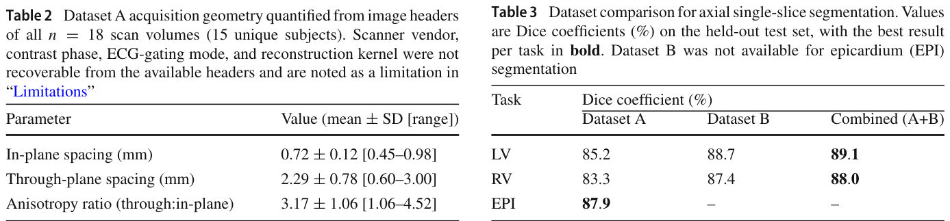
Table 2. Table 2 Dataset A acquisition geometry quantified from image headers of all n = 18 scan volumes (15 unique subjects). Scanner vendor, contrast phase, ECG-gating mode, and reconstruction kernel were not recoverable from the available headers and are noted as a limitation in “Limitations”解説: データセットAの全18スキャンボリューム(15名の固有の対象者)の画像ヘッダーから定量化された取得幾何学的特性です。面内間隔、スライス間隔、異方性比の平均値、標準偏差、範囲が示されています。
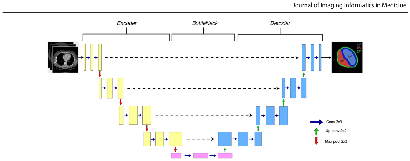
Figure 3. Fig. 3 Overview of our 2.5D U-Net. A small stack of adjacent slices is concatenated as input channels. The encoder extracts multi-scale features, the decoder outputs pixel-wise masks, attention-gated skip解説: 本研究で使用された2.5D U-Netの概要図です。隣接するスライスの小さなスタックが入力チャネルとして連結されます。エンコーダーはマルチスケール特徴を抽出し、デコーダーはピクセルごとのマスクを出力します。アテンションゲート付きスキップコネクションは無関係な活性化を抑制し、ディープスーパービジョンはトレーニング中に補助出力を提供して最適化を安定させます。
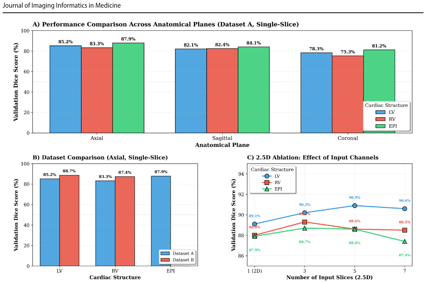
Table 3. Table 3 Dataset comparison for axial single-slice segmentation. Values are Dice coefficients (%) on the held-out test set, with the best result per task in bold. Dataset B was not available for epicardium (EPI) segmentation解説: 軸位シングルスライスセグメンテーションのデータセット比較です。手動(データセットA)、公開(データセットB)、および結合(A+B)データセットを用いた場合の、LV、RV、EPIに対するDice係数(%)が示されており、タスクごとの最良結果が太字で強調されています。
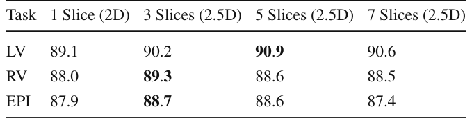
Table 4. Table 4 2.5D ablation study on axial segmentation. Models were trained without augmentation, on the combined Dataset A and B pool for LV and RV and on Dataset A alone for EPI, which has no Dataset B labels. Values are Dice coefficients (%) on the held-out test set, with the best result per task in bold解説: 軸位セグメンテーションにおける2.5Dアブレーション研究です。データ拡張なしで学習されたモデルについて、LV、RV、EPIに対し、1スライス(純粋2D)、3スライス、5スライス、7スライス(2.5D)の各入力設定におけるDice係数(%)が示されています。タスクごとの最良結果が太字で強調されています。
Table 5. Table 5 Impact of data augmentation on 2D segmentation performance. Dice coefficients (%) reported for EPI, LV, and RV with and without augmentation on axial single-slice models trained on Dataset A. Best results per structure in bold解説: データ拡張が2Dセグメンテーション性能に与える影響です。軸位シングルスライスモデルをデータセットAで学習した場合の、EPI、LV、RVのDice係数(%)が、データ拡張なしとデータ拡張ありで比較されています。構造ごとの最良結果が太字で強調されています。
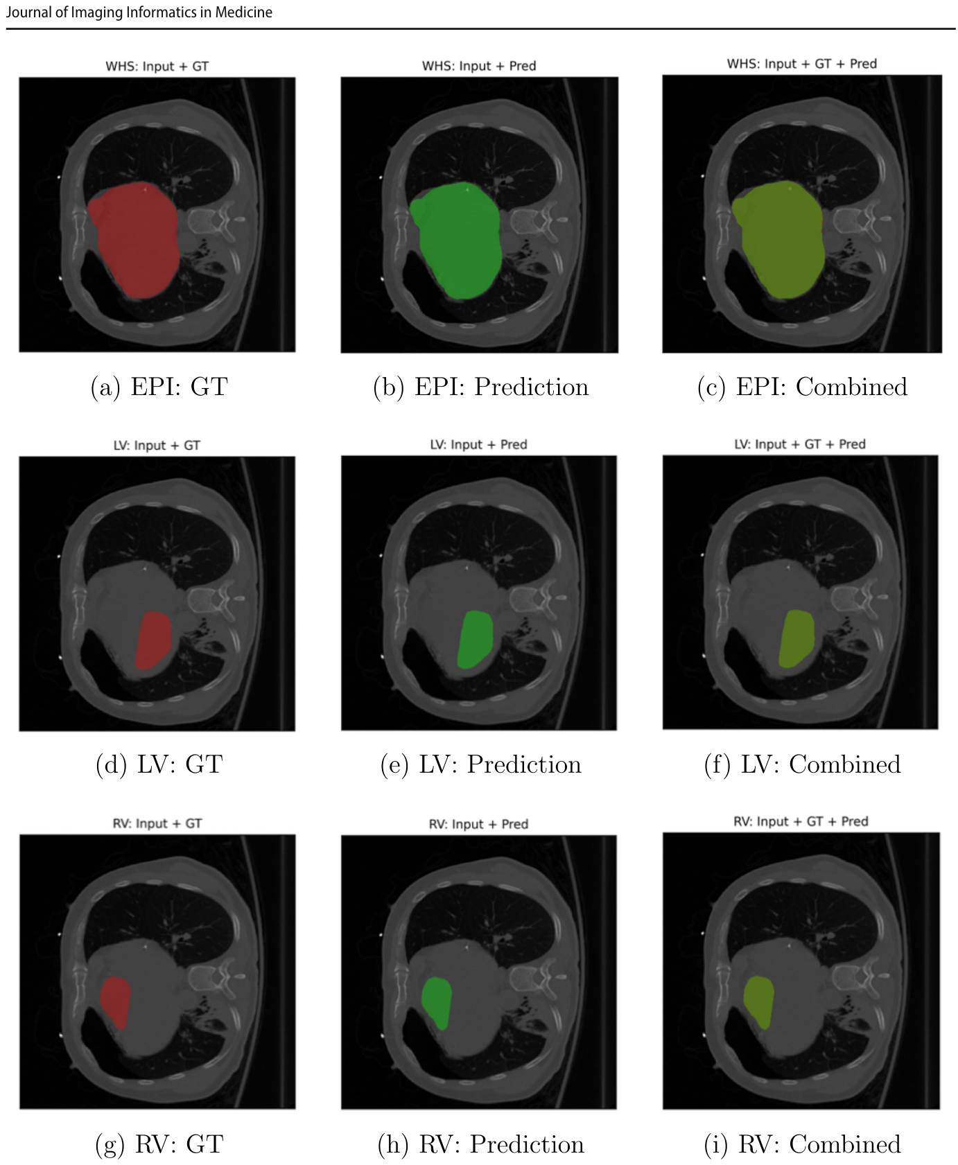
Figure 5. Fig. 5 Qualitative 2D segmentation results on representative axial CT slices. Top row, epicardium (EPI); middle row, left ventricle (LV); bot- tom row, right ventricle (RV). The left column shows ground truth overlays (red), the middle column shows model predictions (green), and解説: 代表的な軸位CTスライスにおける2Dセグメンテーションの定性的結果です。上段は心外膜(EPI)、中段は左心室(LV)、下段は右心室(RV)を示します。左列はグラウンドトゥルースのオーバーレイ(赤)、中列はモデル予測(緑)、右列は結合比較(黄色は一致を示す)です。予測とグラウンドトゥルースが密接に一致していることが視覚的に確認できます。
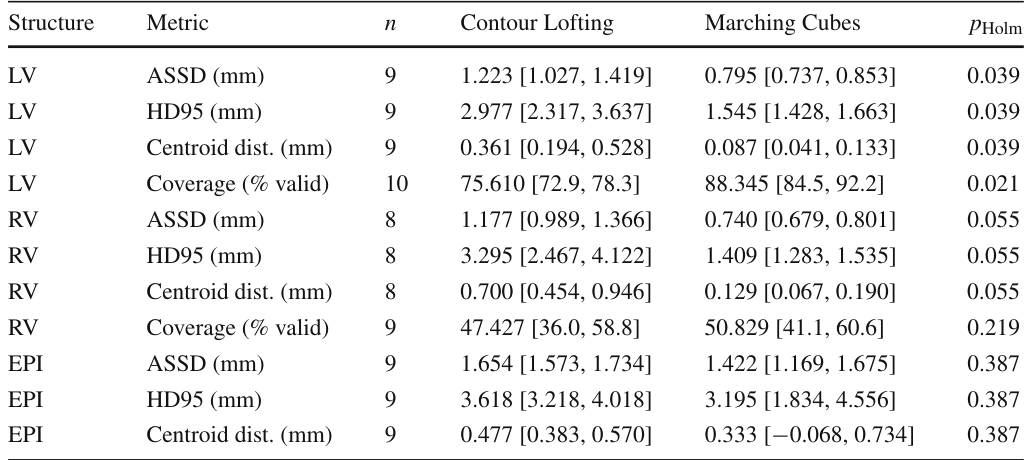
Table 6. Table 6 Reconstruction accuracy, Contour Lofting vs. Marching Cubes, with paired Wilcoxon signed-rank tests (Holm-corrected). Values are mean [95% CI, normal approx.]; tests on the per-structure scan intersection (n). Each of the n scans in every row comes from a distinct subject. Coverage is the percentage of endocardial vertices yielding a valid thickness解説: 輪郭ロフティングとマーチングキューブ法による再構築精度を比較した表です。LV、RV、EPIの各構造について、平均対称表面距離(ASSD)、95パーセンタイルハウスドルフ距離(HD95)、重心距離、カバレッジ(有効な厚みを生じる内膜頂点の割合)などの指標が示されています。また、対応するWilcoxon符号順位検定とHolm補正後のp値も含まれています。
Table 8. Table 8 Regional wall-thickness agreement (mm), reported as the mean of per-scan medians with a 95% confidence interval from the normal approximation. MAE is the mean absolute error, bias
Table 7. Table7 Sensitivityofthicknesstopercentileclipping(MarchingCubes surfaces). Reporting clipped (valid-vertex) vs. un-clipped (all-vertex) statistics and the fraction of vertices removed. The high RV removal解説: パーセンタイルクリッピングに対する壁厚の感度を示した表です。マーチングキューブ法で再構築された表面について、クリッピングされた(有効な頂点)統計とクリッピングされていない(全頂点)統計、および除去された頂点の割合が報告されています。RVの除去割合が高いのは、壁が薄いため、または品質管理によって拒否されたためとされています。




コメントを残す