どうも、Beyond the Pixelです。糖尿病性足潰瘍や静脈性下腿潰瘍、褥瘡など、治りにくい慢性創傷は、多くの対象者を苦しめ、医療費を増大させています。これらの創傷では、正常な治癒プロセスが滞ることが多く、創傷表面には生きている組織と死んだ組織が混在します。創傷底にどのような組織が存在し、その割合がどのように変化するかを評価することは、治癒の進行状況を把握し、デブリードマン(死んだ組織の除去)などの治療方針を決定する上で不可欠です。
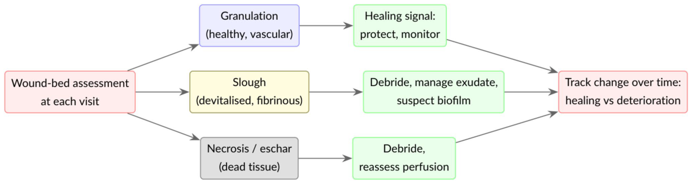
Figure 1. Fig. 1 The wound bed tissues and their evolution drive clinical deci- sions. At each visit, the clinician identifies granulation, slough, and necrotic tissue and, above all, judges how their proportions change over time; that trajectory guides debridement, dressing choice and解説: この図は、創傷底組織とその変化が臨床的判断をどのように推進するかを示すフローチャートです。専門家は各診察時に、肉芽組織、スラフ、壊死組織を識別し、特にそれらの割合が時間とともにどう変化するかを評価します。その変化の軌跡が、デブリードマン(死んだ組織の除去)、ドレッシングの選択、治療の強化などの介入を導きます。本研究の課題は、これらの組織を自動的かつ再現性高く定量化し、治癒の軌跡を客観的に追跡することです。
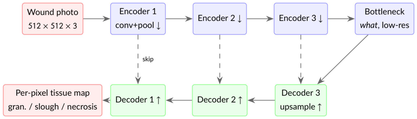
Figure 2. Fig. 2 Encoder–decoder for semantic segmentation. The encoder progressively compresses the image into abstract features (learn- ing what tissue is present), and the decoder upsamples them back to full resolution to label every pixel (recovering where). Skip connec-解説: セマンティックセグメンテーションのためのエンコーダー・デコーダー構造を示しています。エンコーダーは画像を抽象的な特徴へと段階的に圧縮し(どの組織が存在するかを学習)、デコーダーはそれらの特徴を元の解像度に戻し、ピクセルごとにラベル付けします(どこに組織があるかを復元)。U-Netのように、スキップ接続(点線)は、ダウンサンプリング中に失われた細かい空間情報を渡します。DeepLabV3+は、アトラス畳み込みとマルチスケールプーリングを用いて解像度を維持します。
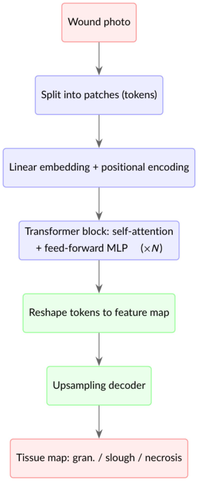
Figure 3. Fig. 3 Transformer encoder for segmentation. The image becomes a sequence of patch tokens; self-attention models the relationships between all patches at once, the block repeats, and the tokens are reshaped and upsampled into a per-pixel map. Plain Vision Trans- formers (ViT, SETR) use a single-scale token grid, whereas Seg- Former produces multi-scale features like a CNN解説: セグメンテーションのためのトランスフォーマーエンコーダーの仕組みを示しています。画像はパッチトークンのシーケンスに分割され、セルフアテンションメカニズムによってすべてのパッチ間の関係が同時にモデル化されます。このブロックが複数回繰り返され、トークンは再形成されてピクセルごとのマップにアップサンプリングされます。Plain Vision Transformers(ViT、SETR)は単一スケールのトークングリッドを使用し、SegFormerはCNNのようにマルチスケール特徴を生成します。
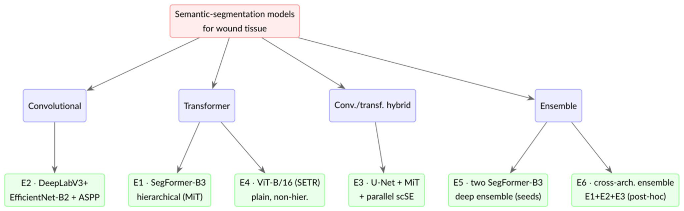
Figure 4. Fig. 4 The architectures, by family. Experiments E1–E5 map onto the convolutional, transformer, hybrid and ensemble families; E6 is a post-hoc cross-architecture ensemble that averages the convolu- tional and transformer single models (E1–E3), combining diversity of architecture rather than of random seed (Section " Cross-Architecture解説: 本研究で評価されたセマンティックセグメンテーションモデルのアーキテクチャをファミリー別に分類して示しています。実験E1〜E5は、畳み込み、トランスフォーマー、ハイブリッド、アンサンブルのファミリーに対応しています。E6は、畳み込みおよびトランスフォーマーの単一モデル(E1〜E3)を平均化するポストホックなクロスアーキテクチャアンサンブルを表しており、ランダムシードの多様性ではなくアーキテクチャの多様性を組み合わせています。これらをほぼ共通のプロトコルで比較することで、創傷組織セグメンテーションにおけるアーキテクチャの影響を推定します。
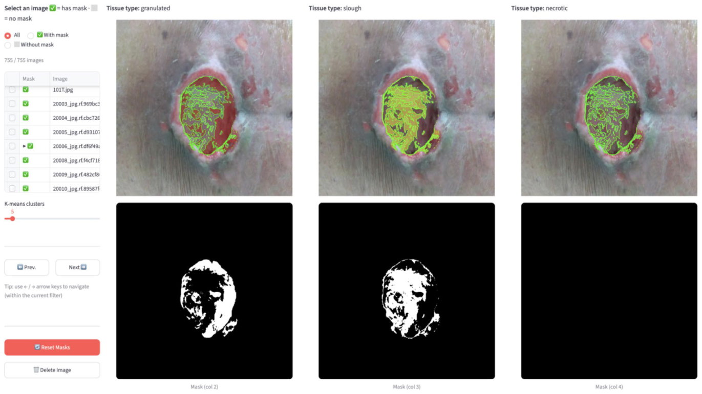
Figure 6. Fig. 6 The custom in-house annotation tool (local HTML/JS app). The clinician opens a wound photo; the app automatically applies k-means colour clustering to segment the wound by colour (the clus- ter count k is adjustable to increase resolution). The photo is repli- cated across three columns, one per tissue colour, red (granulation), yellow (slough), black (necrotic/eschar); clicking a clustered region解説: カスタム開発された社内アノテーションツール(ローカルHTML/JSアプリ)のスクリーンショットです。専門家が創傷写真を開くと、アプリは自動的にK-meansカラークラスタリングを適用して、創傷を色でセグメント化します。写真は赤(肉芽組織)、黄(スラフ)、黒(壊死組織/痂皮)の3つの組織色ごとに3つのカラムに複製され、クラスター化された領域をクリックすることで、その領域全体にカラムのクラスが割り当てられます。このクラスター支援型ワークフローは、手書きでの線引きと比較してラベリングを大幅に加速させます。
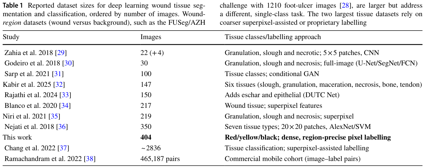
Table 1. Table 1 Reported dataset sizes for deep learning wound tissue seg- mentation and classification, ordered by number of images. Wound- region datasets (wound versus background), such as the FUSeg/AZH解説: 深層学習を用いた創傷組織セグメンテーションおよび分類に関する公開データセットのサイズを、画像数順にまとめた表です。本研究のデータセットは404枚の画像を含み、赤/黄/黒の組織に対して密で領域精度の高いピクセルラベリングが施されています。多くの既存研究が数十枚から数百枚の画像を使用しており、本研究のデータセットはピクセルレベルの創傷組織セグメンテーションとしては比較的規模が大きいことが示されています。
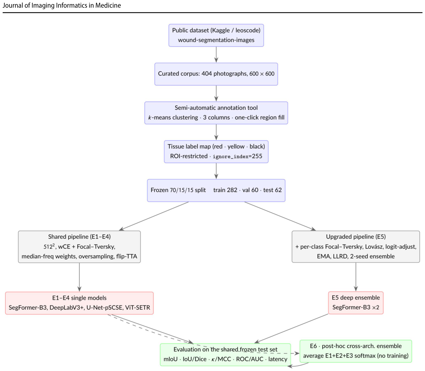
Figure 13. Fig. 13 Experimental pipeline. One curated, version-locked dataset and a single frozen split feed a shared training and evaluation pro- tocol; experiments E1–E4 vary the network under this shared frame- work (with only minor, documented per-model tuning of the loss asymmetry, class weights and optimiser settings; Table 2), while E5
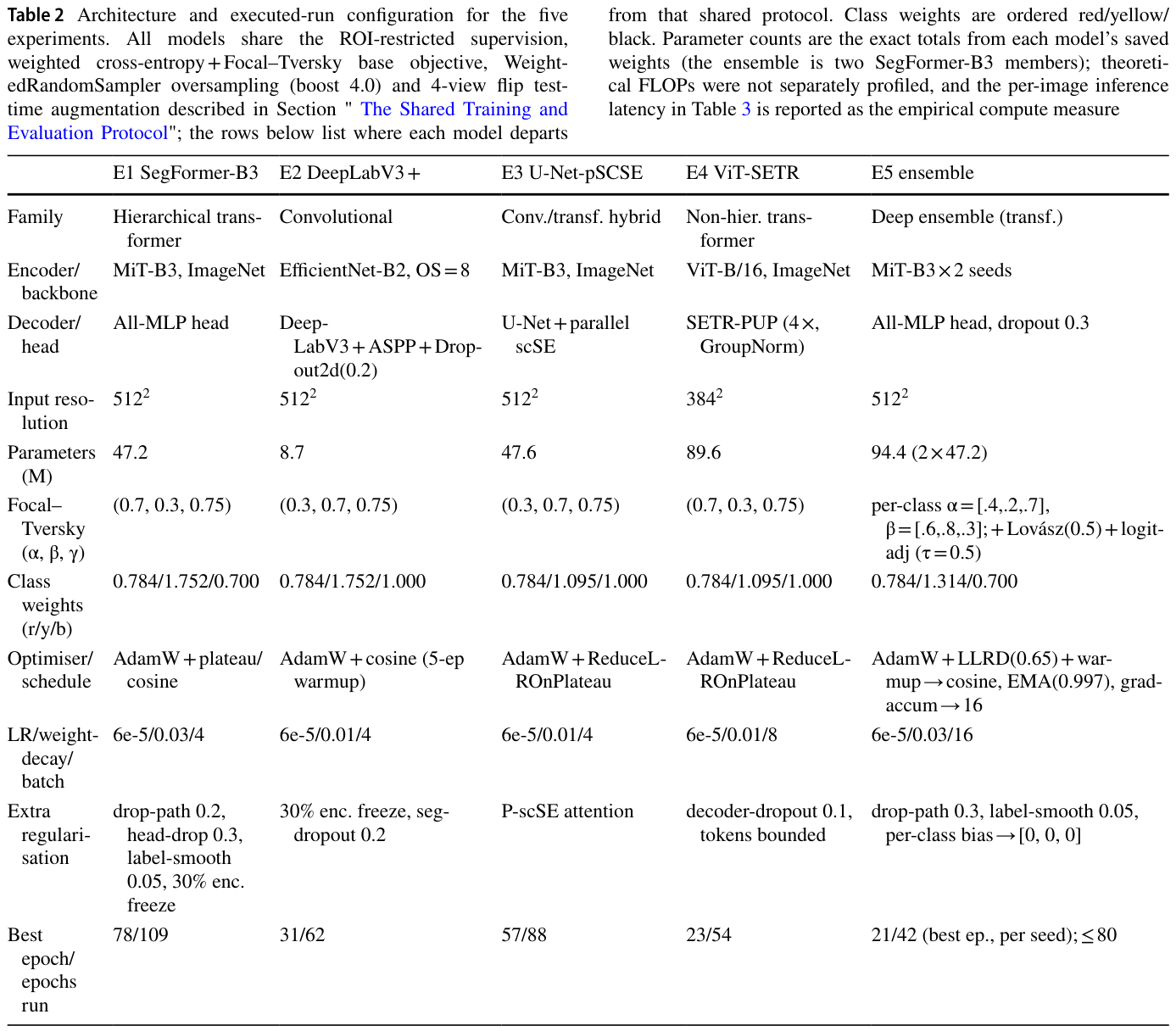
Table 2. Table 2 Architecture and executed-run configuration for the five experiments. All models share the ROI-restricted supervision, weighted cross-entropy + Focal–Tversky base objective, Weight- edRandomSampler oversampling (boost 4.0) and 4-view flip test- time augmentation described in Section " The Shared Training and Evaluation Protocol"; the rows below list where each model departs解説: 評価された5つの実験におけるアーキテクチャと実行設定の構成をまとめた表です。全てのモデルはROIに限定された教師あり学習、重み付き交差エントロピー+Focal-Tverskyの基本目的関数、WeightedRandomSamplerによるオーバーサンプリング、4ビューフリップテスト時拡張を共有しています。この表は、各モデルが共有プロトコルから逸脱した箇所(Focal-Tverskyの非対称性、クラス重み、オプティマイザ、学習率、正則化など)を詳細に示しています。
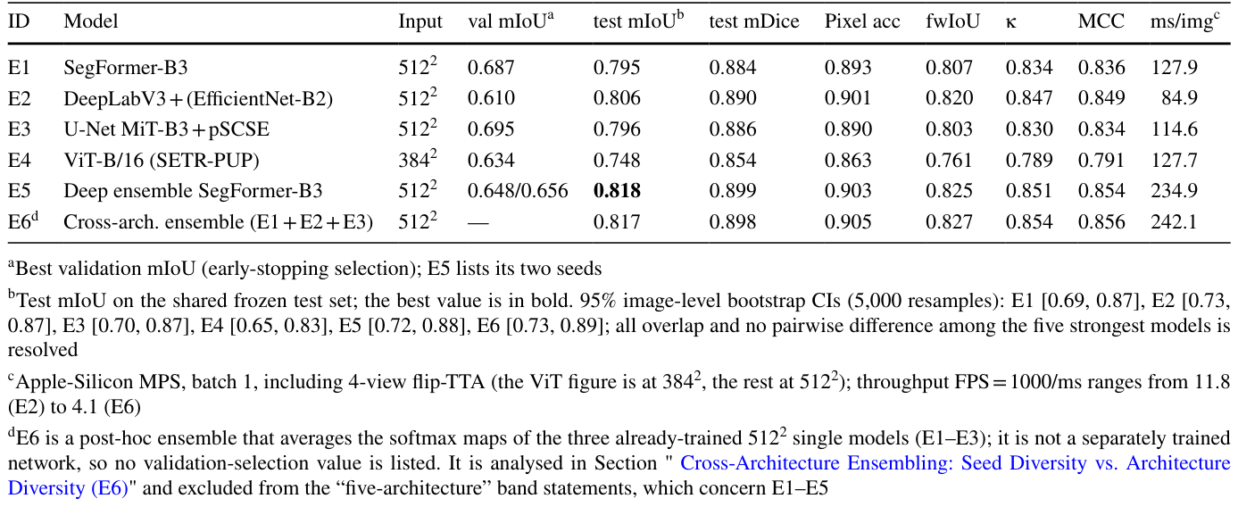
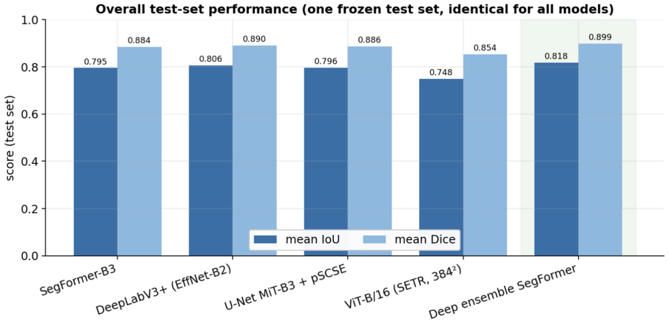
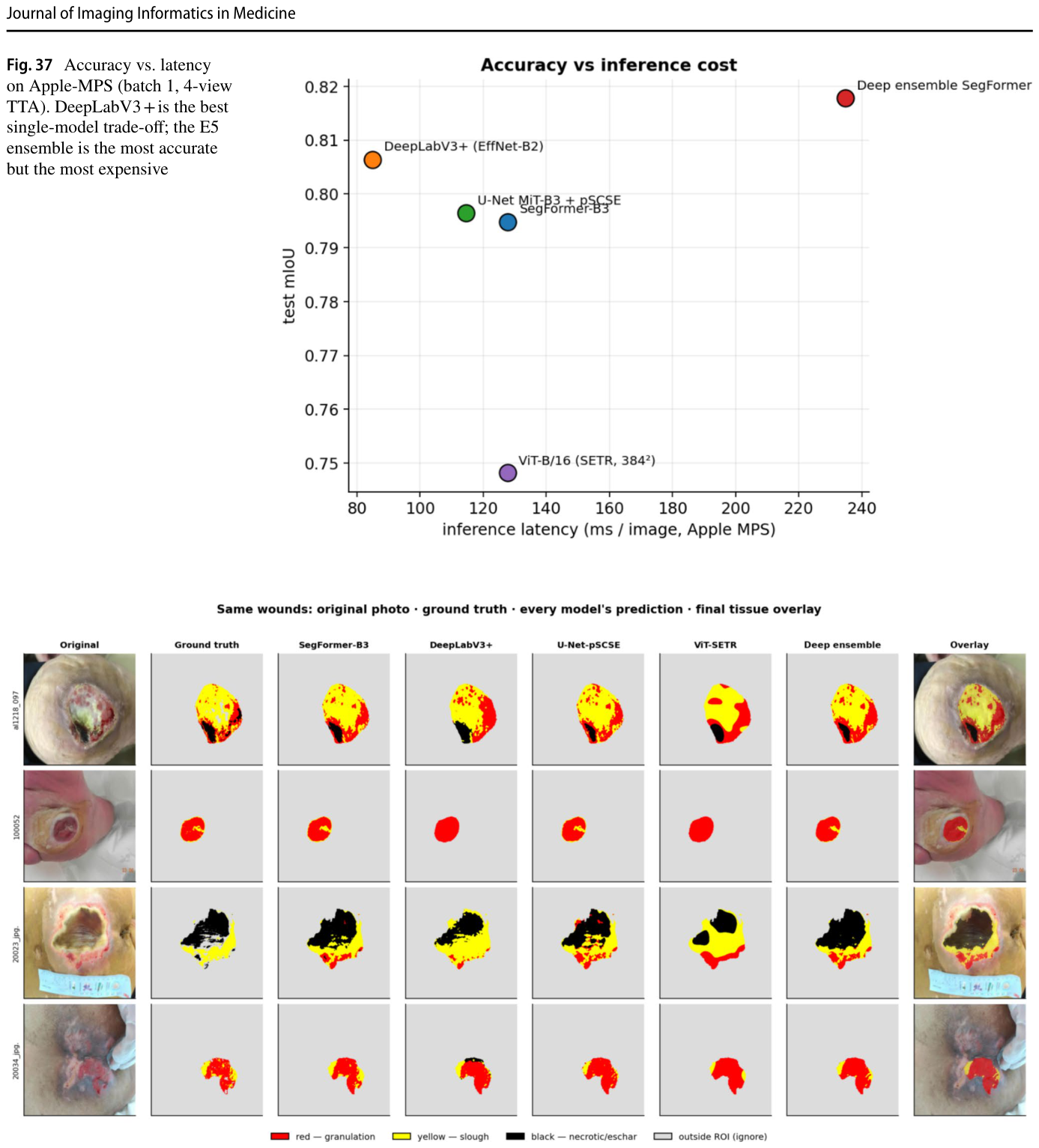
Table 3. Table 3 Overall performance on the shared frozen test set. Primary metric: test mIoU. All models share the same 62-image test set, ROI masks and ignore convention解説: 共通の凍結テストセットにおける全体の性能を示した表です。主要な評価指標はテストmIoU(平均Intersection-over-Union)です。全てのモデルは同じ62枚の画像テストセットで評価されています。最も性能の高いモデル(E5 Deep ensemble SegFormer-B3)は0.818のmIoUを達成しており、最も強力な単一モデル(E2 DeepLabV3+)も0.806と高いスコアを示しています。
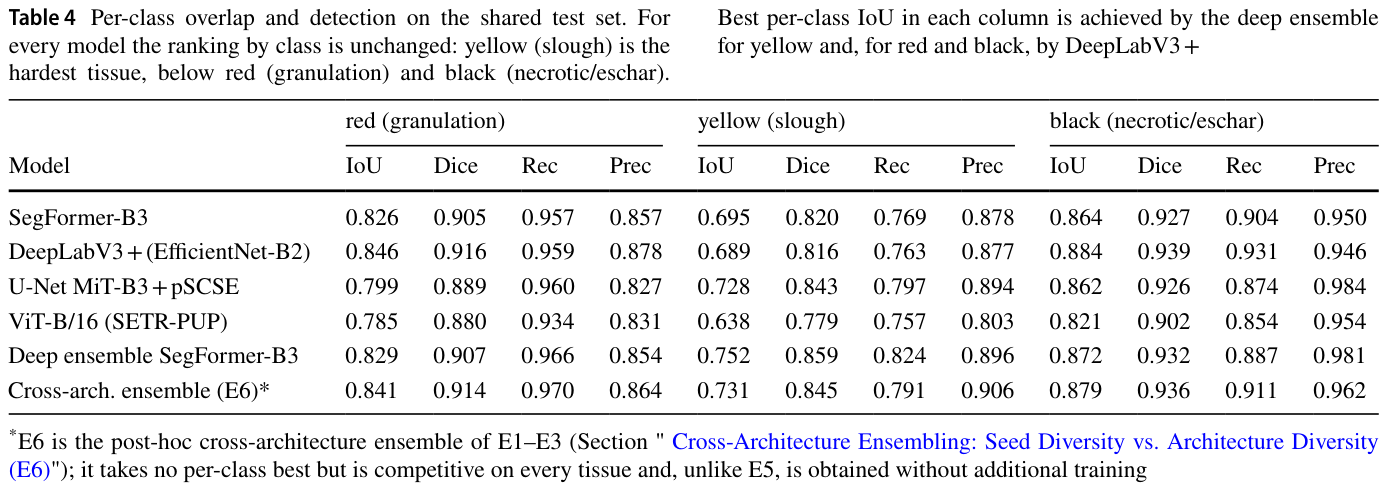
Table 4. Table 4 Per-class overlap and detection on the shared test set. For every model the ranking by class is unchanged: yellow (slough) is the hardest tissue, below red (granulation) and black (necrotic/eschar).解説: 共通テストセットにおけるクラスごとの重複度と検出性能を示した表です。全てのモデルにおいて、クラスによる順位は変わらず、黄色(スラフ)が最も困難な組織であり、次いで赤(肉芽組織)、黒(壊死組織/痂皮)となります。最も高いクラスごとのIoUは、黄色と赤ではDeep ensemble SegFormer-B3が、黒ではDeepLabV3+が達成しています。
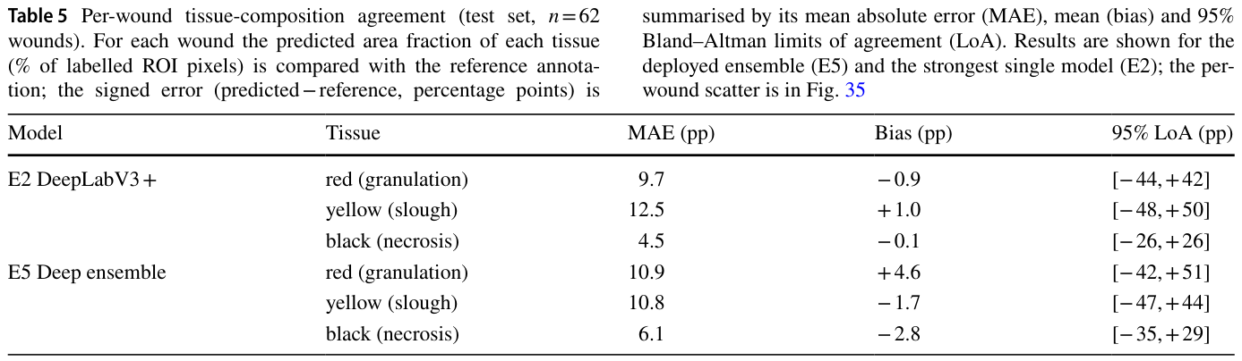
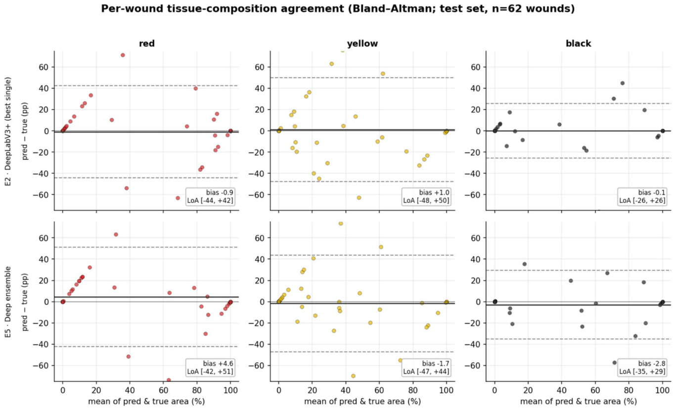
Table 5. Table 5 Per-wound tissue-composition agreement (test set, n = 62 wounds). For each wound the predicted area fraction of each tissue (% of labelled ROI pixels) is compared with the reference annota- tion; the signed error (predicted − reference, percentage points) is解説: テストセット(62創傷)における創傷あたりの組織構成の一致度を示した表です。各創傷について、ラベル付けされたROIピクセルの予測面積割合と参照アノテーションを比較しています。結果は展開されたアンサンブルモデル(E5)と最も強力な単一モデル(E2)について示されており、平均絶対誤差(MAE)、バイアス、95%一致の限界(LoA)が含まれています。スラフ組織の一致の限界が他の組織よりも広いことが示されています。
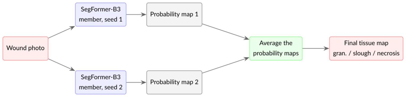
Figure 5. Fig. 5 How a deep ensemble works. The same architecture is trained several times from different random seeds; at inference the members’ probability maps are averaged, so their uncorrelated errors tend to解説: ディープアンサンブルの仕組みを示しています。同じアーキテクチャが異なるランダムシードから複数回訓練され、推論時にはメンバーの確率マップが平均化されます。これにより、相関のない誤差が相殺され、合意されたシグナルが強化されます。展開されたモデル(E5)は、2つのSegFormer-B3メンバーの予測を平均化します。
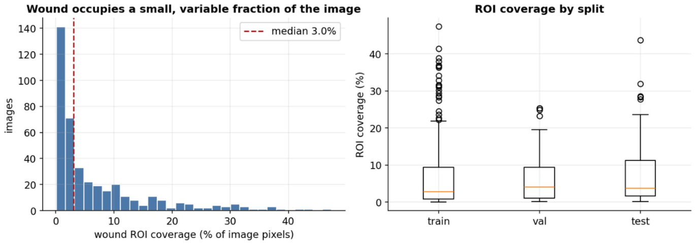
Figure 7. Fig. 7 Wound ROI coverage as a fraction of the image (left) and by split (right)解説: 創傷の関心領域(ROI)が画像全体に占める割合(左)と、訓練、検証、テストの各データ分割におけるROIカバー率(右)を示しています。左のグラフは、創傷ROIが画像ピクセルの平均7.0%、中央値3.0%と、画像のごく一部であることがわかります。右のボックスプロットは、各分割データセットにおけるROIカバー率の分布を示しています。
Figure 8
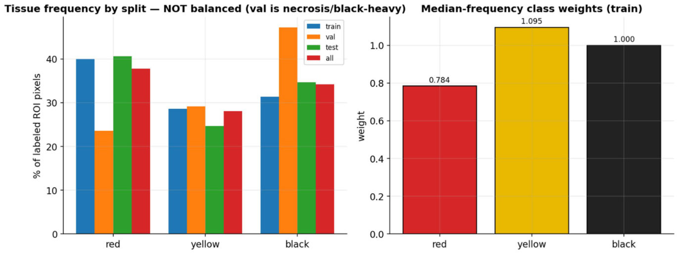
Figure 8. Fig. 8 Tissue pixel frequency per split (left) and the median frequency class weights used in training (right)
Figure 9
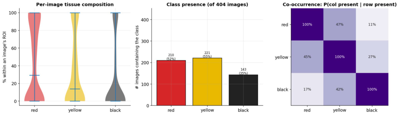
Figure 9. Fig. 9 Per-image tissue composition (left), class presence (centre) and image-level co-occurrence (right)
Figure 10
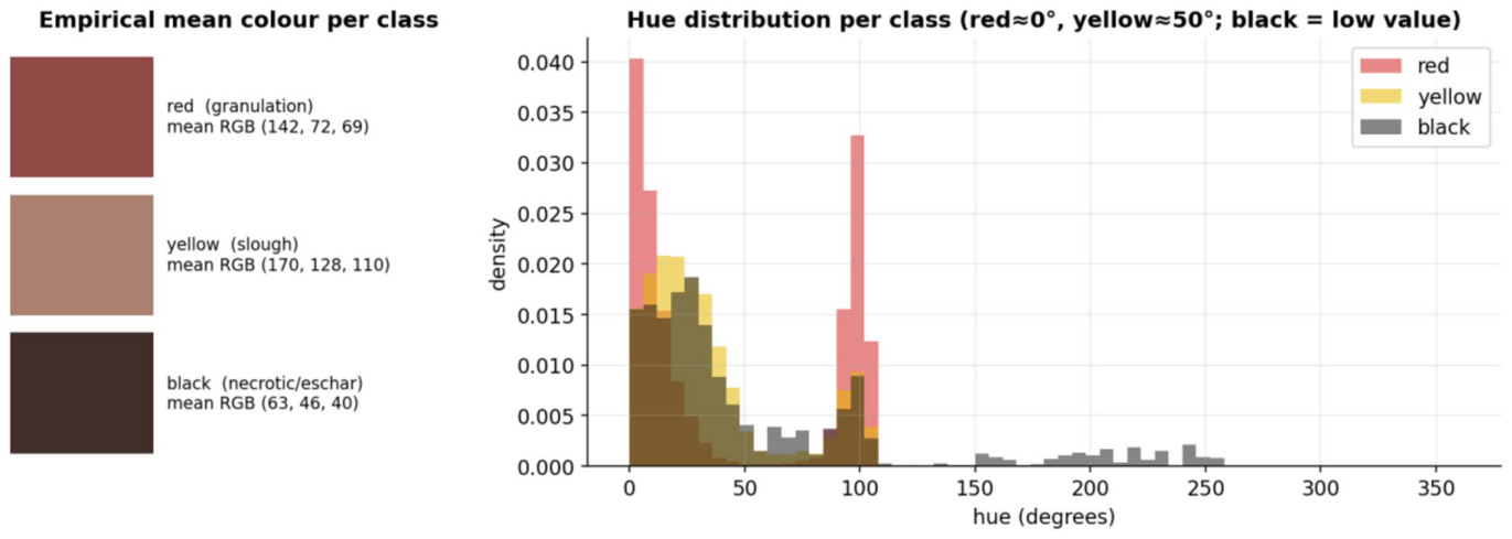
Figure 10. Fig. 10 Empirical mean colour per class (left) and per-class hue distributions (right)
Figure 12
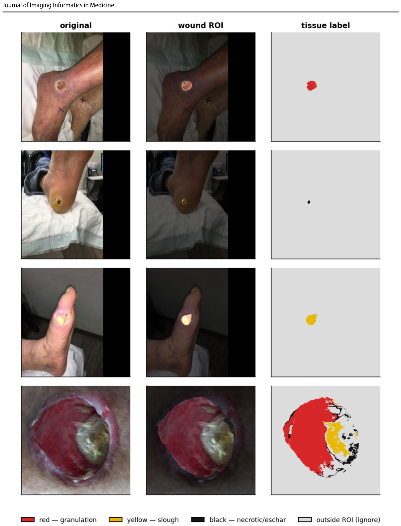
Figure 12. Fig. 12 Representative test cases: the original photo, the wound ROI (background dimmed) and the colour-coded tissue label map
Figure 14
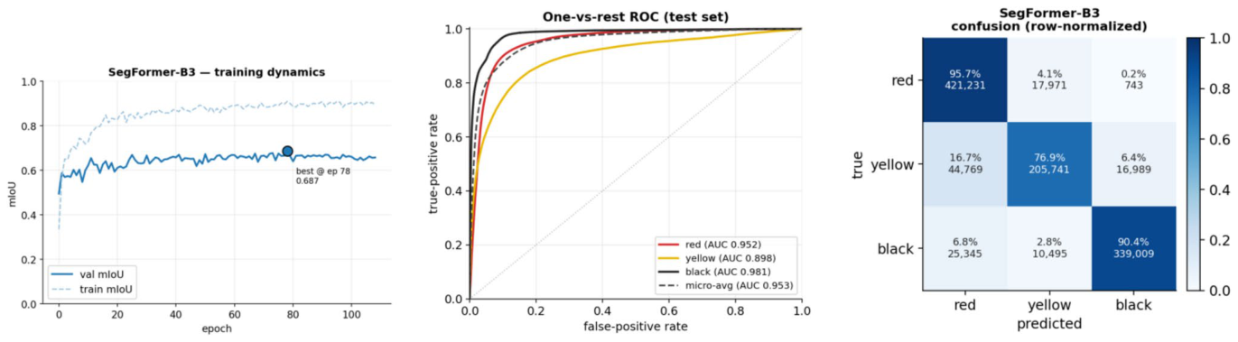
Figure 14. Fig. 14 E1 (SegFormer-B3) diagnostics. Left: training dynamics (solid = validation, dashed = train; • marks the selected best-val- idation-mIoU epoch). Centre: one-vs-rest ROC on the test set from
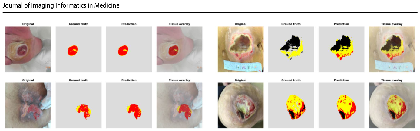
Figure 15
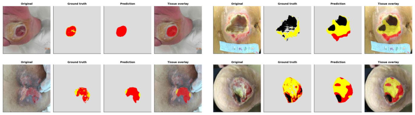
Figure 15. Fig. 15 E1 (SegFormer-B3) qualitative test cases. From left within each panel: the original wound photo, the ground truth tissue map, the model’s prediction, and the tissue overlaid on the photo. The
Figure 16
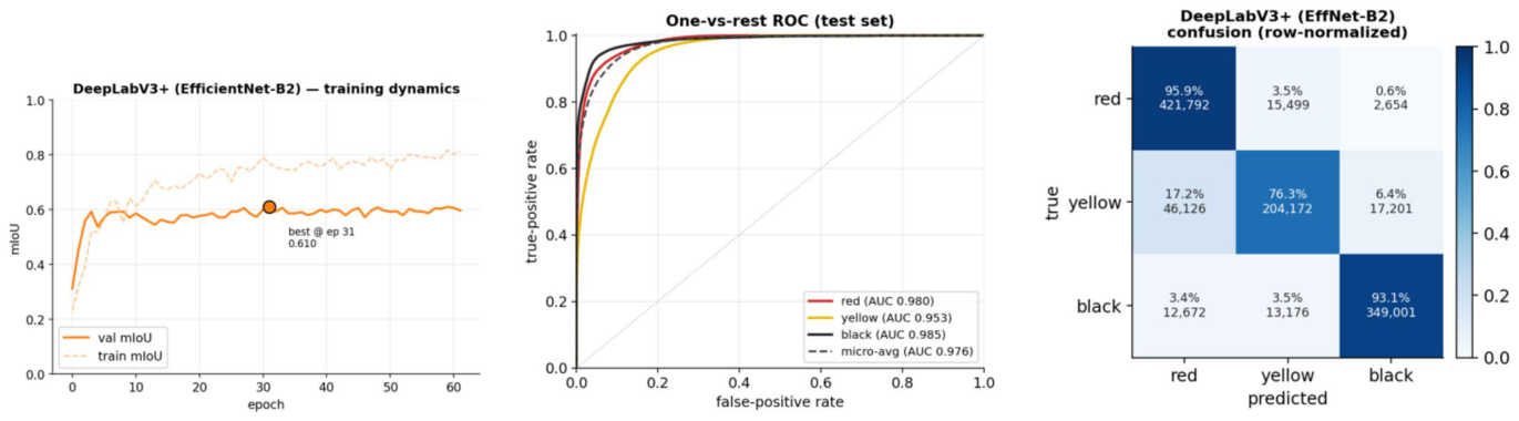
Figure 16. Fig. 16 E2 (DeepLabV3 +) diagnostics. Left: training dynamics (solid = validation, dashed = train; • marks the selected best-val- idation-mIoU epoch). Centre: one-vs-rest ROC on the test set from
Figure 17
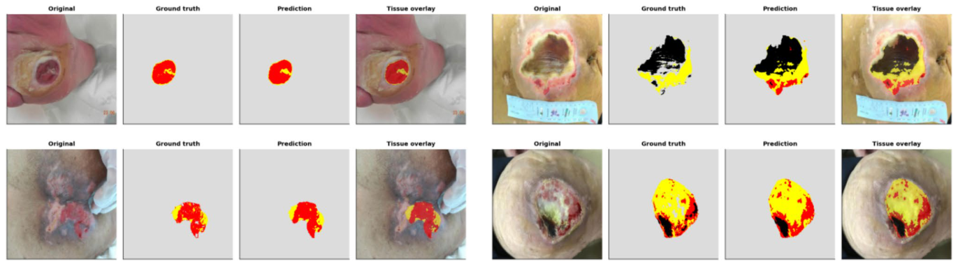
Figure 17. Fig. 17 E2 (DeepLabV3 +) qualitative test cases. From left within each panel: the original wound photo, the ground truth tissue map, the model’s prediction, and the tissue overlaid on the photo. The
Figure 18
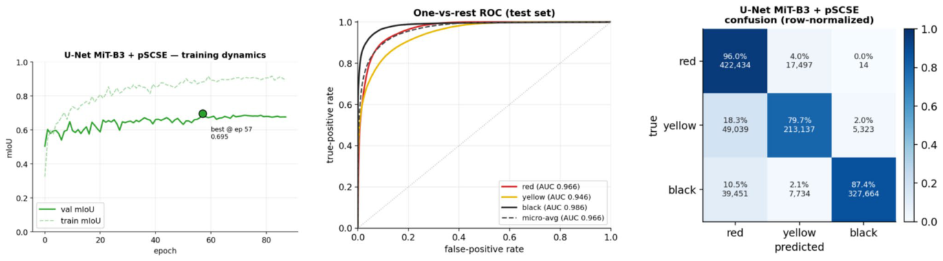
Figure 18. Fig. 18 E3 (U-Net MiT-B3 + pSCSE) diagnostics. Left: training dynamics (solid = validation, dashed = train; • marks the selected best-validation-mIoU epoch). Centre: one-vs-rest ROC on the test set
Figure 19
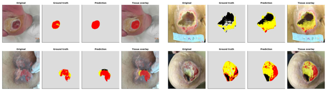
Figure 19. Fig. 19 E3 (U-Net MiT-B3 + pSCSE) qualitative test cases. From left within each panel: the original wound photo, the ground truth tissue map, the model’s prediction, and the tissue overlaid on the photo. The
Figure 20
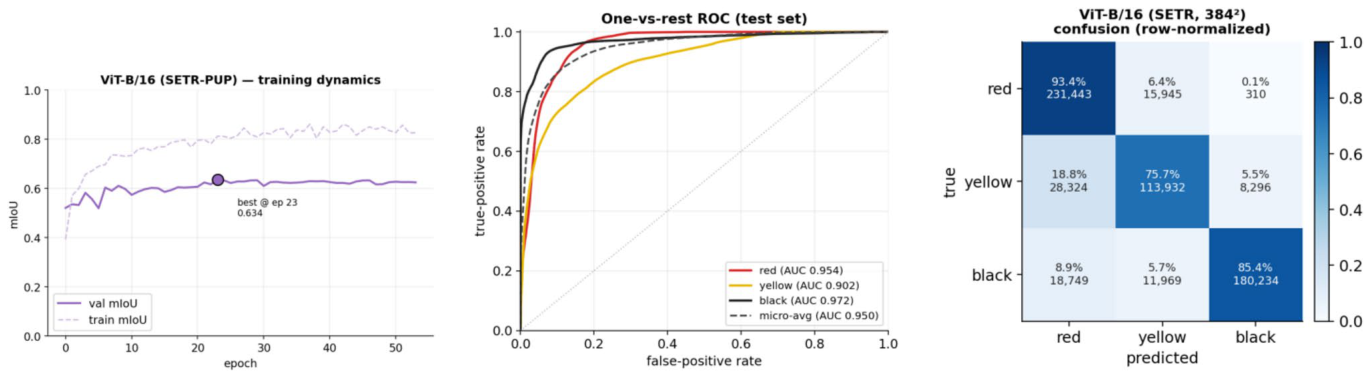
Figure 20. Fig. 20 E4 (ViT-B/16, SETR-PUP) diagnostics. Left: training dynamics (solid = validation, dashed = train; • marks the selected best-validation-mIoU epoch). Centre: one-vs-rest ROC on the test set
Figure 21
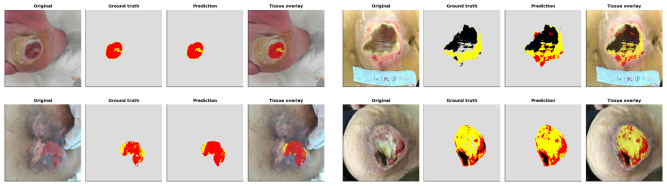
Figure 21. Fig. 21 E4 (ViT-B/16, SETR-PUP) qualitative test cases. From left within each panel: the original wound photo, the ground truth tissue map, the model’s prediction, and the tissue overlaid on the photo. The
Figure 22
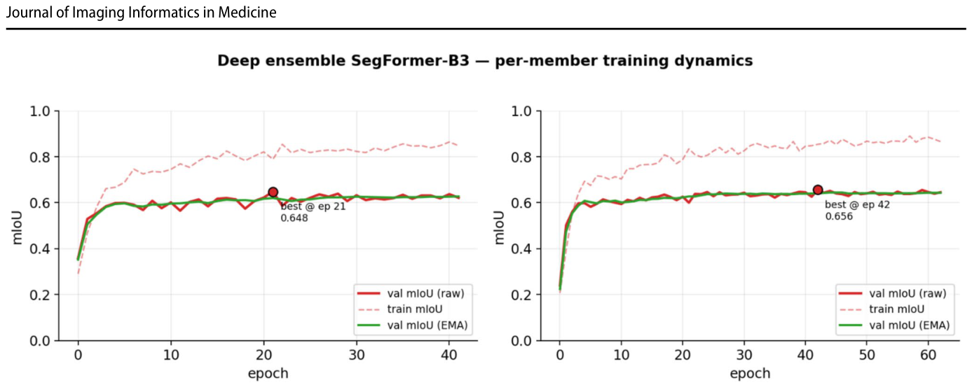
Figure 22. Fig. 22 E5 (deep ensemble) per-member training dynamics of the two seeds (42 and 1234): validation mIoU on the raw weights (solid), training mIoU (dashed) and validation mIoU on the EMA weights (green); • marks the selected best-validation epoch. Both members
Figure 23
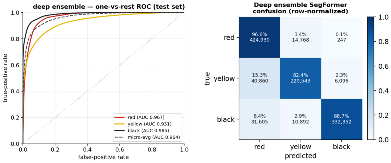
Figure 23. Fig. 23 E5 (deep ensemble) test diagnostics. Left: one-vs-rest ROC from the per-pixel probabilities (flip-TTA); AUC red 0.967, yellow 0.931, black 0.985 (micro-average 0.964); slough (yellow) is the low-
Figure 24
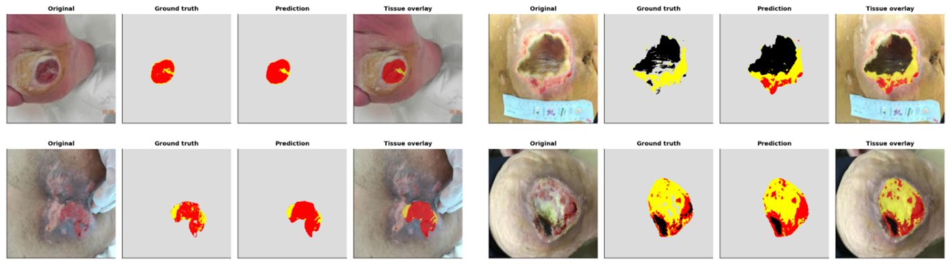
Figure 24. Fig. 24 E5 (deep ensemble) qualitative test cases. From left within each panel: the original wound photo, the ground truth tissue map, the model’s prediction, and the tissue overlaid on the photo. The
Figure 25
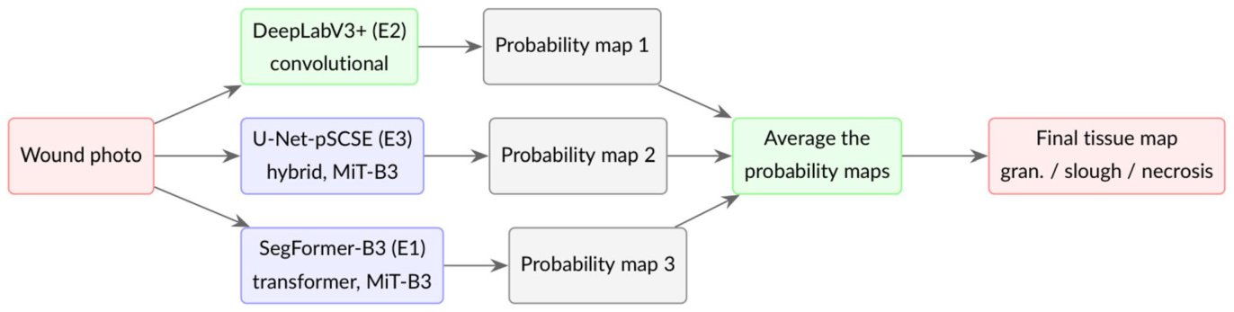
Figure 25. Fig. 25 How the cross-architecture ensemble (E6) works. Three already-trained, architecturally distinct single models, a convolu- tional network (DeepLabV3 +, green) and two Mix-Transformer models (SegFormer-B3 and the U-Net-pSCSE hybrid, blue), process the photo; their flip-TTA probability maps are averaged post hoc,
Figure 26
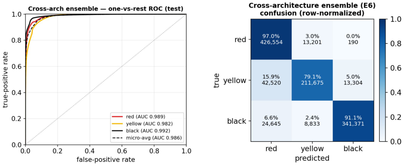
Figure 26. Fig. 26 E6 (cross-architecture ensemble) test diagnostics. Left: one- vs-rest ROC from the per-pixel probabilities (flip-TTA); AUC red 0.989, yellow 0.982, black 0.992 (micro-average 0.986). Right: row- normalised confusion matrix (diagonal = per-class recall). Averaging
Figure 27
Figure 27. Fig. 27 E6 (cross-architecture ensemble) qualitative test cases. From left within each panel: the original wound photo, the ground truth tis- sue map, the model’s prediction, and the tissue overlaid on the photo.
Figure 28
Figure 28. Fig. 28 Overall test-set mIoU and mDice per experiment, on one frozen test set identical for every model (E5 highlighted). All models lie within 0.748–0.818 mIoU; the deep ensemble leads narrowly
Figure 29
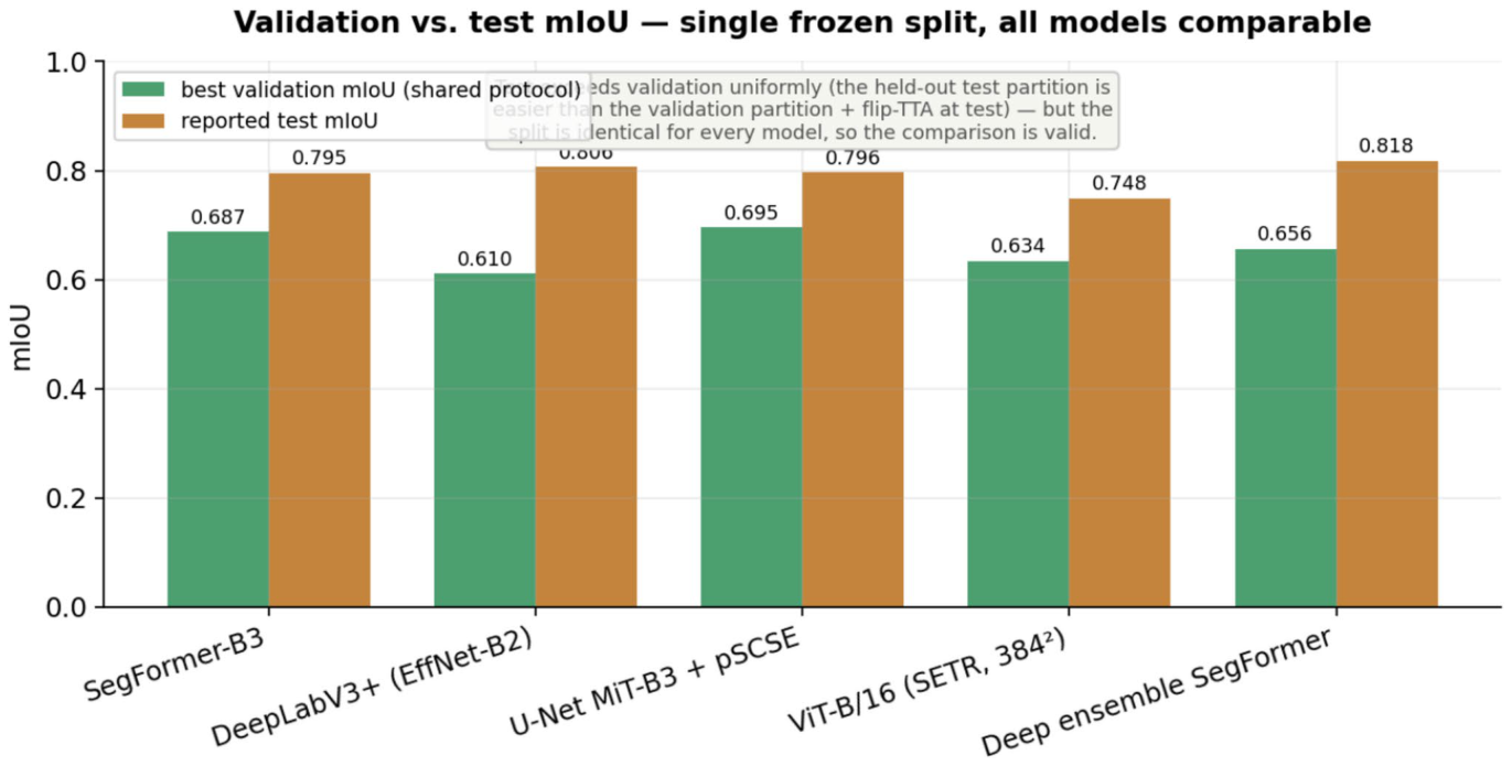
Figure 29. Fig. 29 Validation vs. test mIoU. Test exceeds validation by a fairly uniform + 0.10–0.20 for every model: the held-out test partition appears easier than the (necrosis-heavy) validation partition and addi- tionally benefits from flip-TTA. Because the split is identical for all models, this shared offset cannot bias the relative cross-model rank-
Figure 30
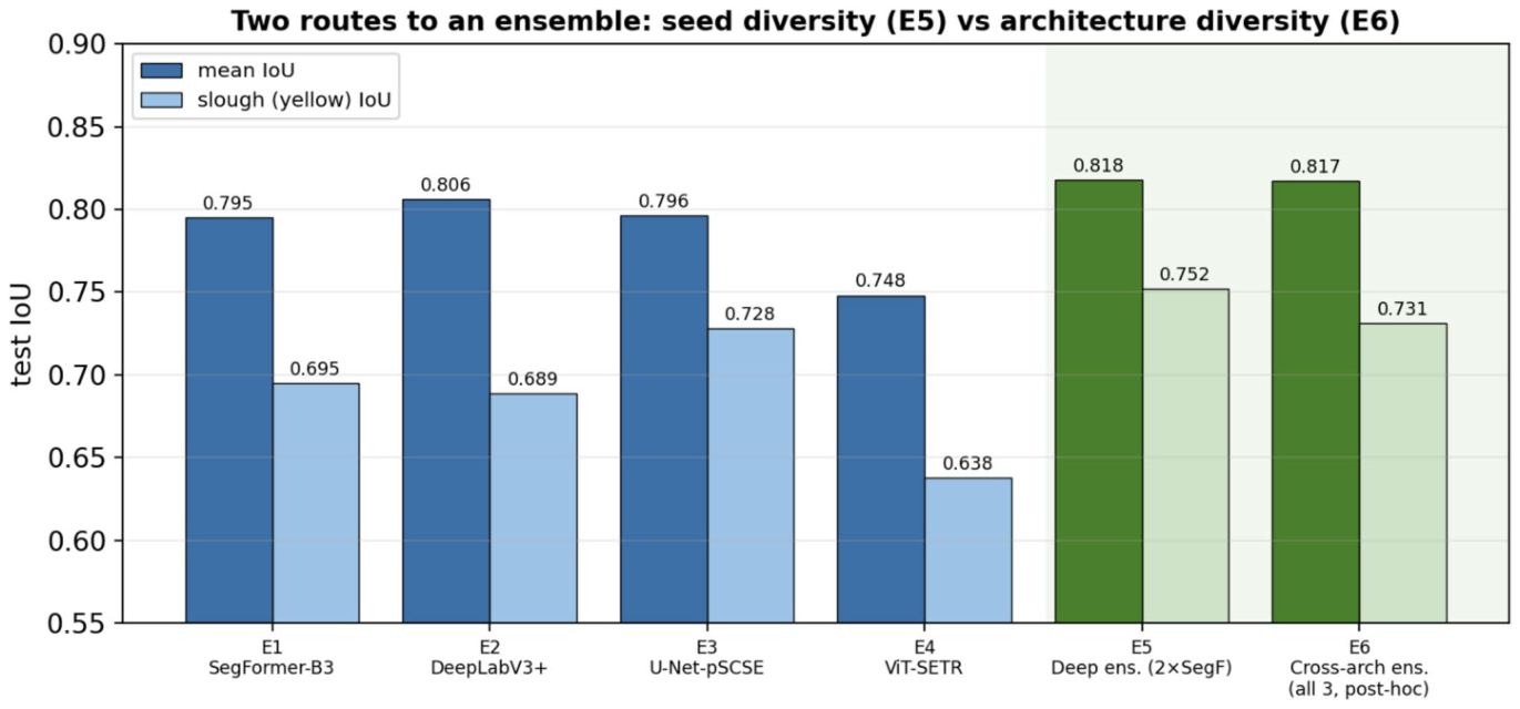
Figure 30. Fig. 30 Two routes to an ensemble. Mean IoU (dark) and slough (yellow) IoU (light) on the shared test set for the four single mod- els (E1–E4), the seed-diversity deep ensemble (E5) and the post-hoc
Figure 31
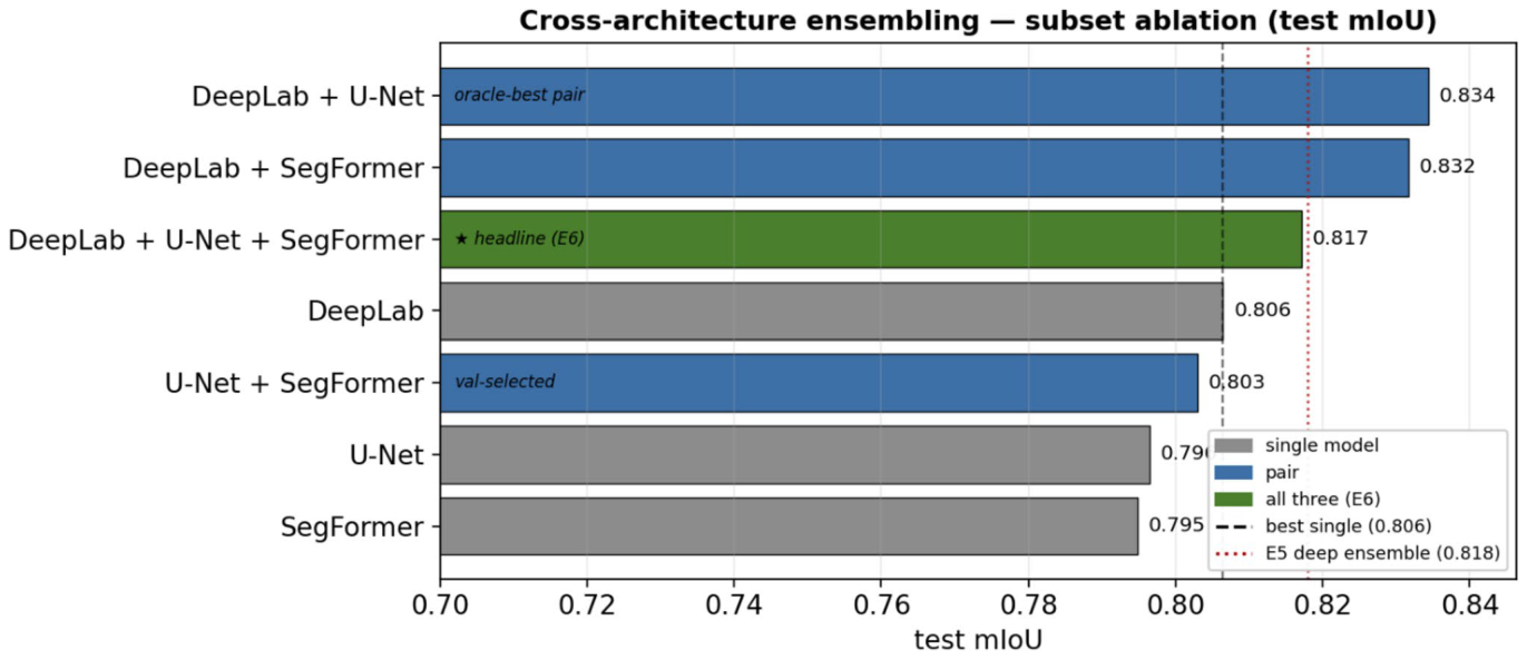
Figure 31. Fig. 31 Subset ablation of the cross-architecture ensemble. Test mIoU of every subset of the three 5122 single models (single = grey, pair = blue, all three = green). Dashed line: best single model; dotted line: the E5 deep ensemble. The principled, selection-free three-way
Figure 32
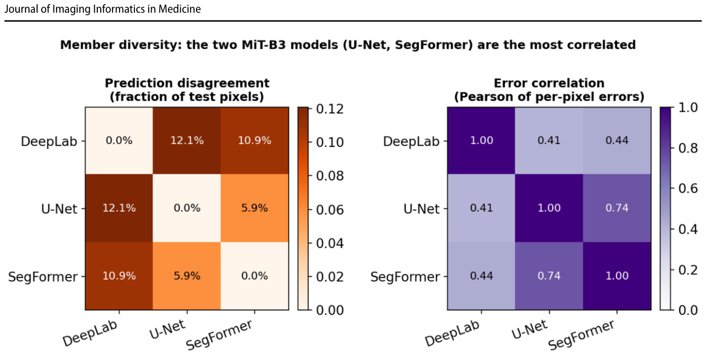
Figure 32. Fig. 32 Member diversity on the test set. Left: pairwise prediction disagreement (fraction of valid pixels where two members’ arg-max labels differ). Right: pairwise Pearson correlation of the members’ per-pixel error indicators. The two MiT-B3 models (U-Net, Seg-
Figure 33
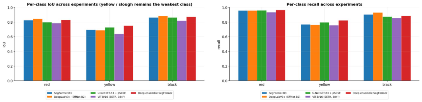
Figure 33. Fig. 33 Per-class IoU (left) and recall (right). Yellow is the weakest class for every model but is now well above 0.6 IoU; the deep ensemble (E5) and U-Net-pSCSE (E3) handle it best
Figure 34
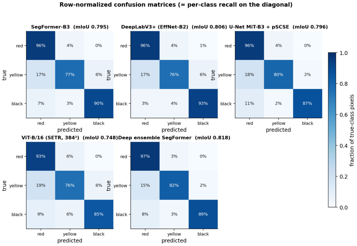
Figure 34. Fig. 34 Row-normalised confusion matrices (diagonal = per-class recall). The residual error is the symmetric yellow ↔ red and yellow ↔ black confusion: ~ 15–18% of true yellow pixels are still assigned to a neighbouring tissue. E5 has the tightest diagonal
Figure 35
Figure 35. Fig. 35 Per-wound tissue-composition agreement (Bland–Altman). For every test wound (n = 62) the predicted minus reference area frac- tion of each tissue (percentage points) is plotted against their mean, for the strongest single model (E2, top row) and the deployed ensem- ble (E5, bottom row). Solid line: mean (bias); dashed lines: 95% lim-
Figure 36
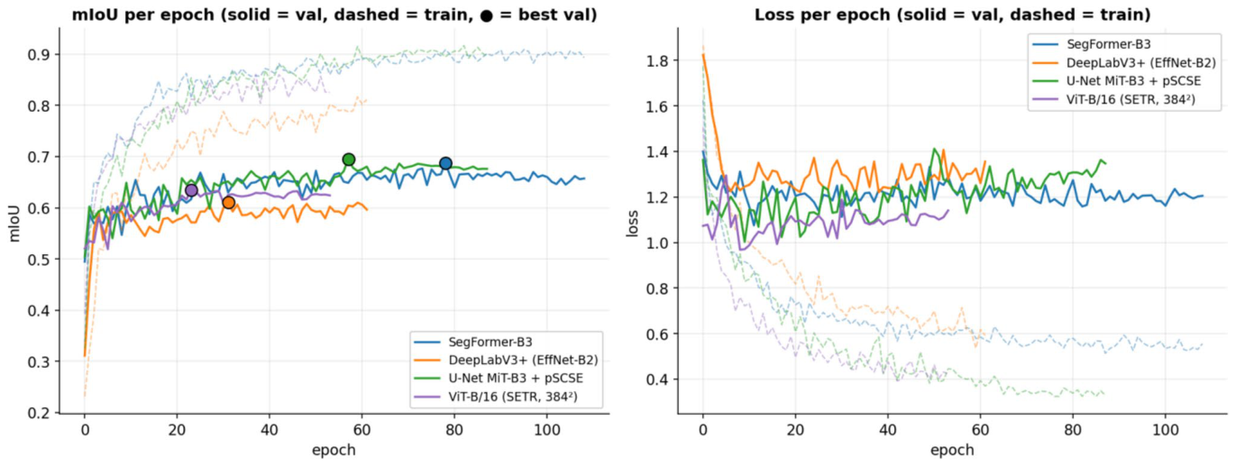
Figure 36. Fig. 36 Per-epoch mIoU and loss (E1–E4). Solid = validation, dashed = train, • = selected (best-val) epoch. Validation now climbs to a stable pla- teau over many epochs rather than collapsing early
Figure 38
Figure 38. Fig. 38 The same four test wounds, shown (left to right) as the origi- nal photo, the ground truth, every model’s prediction, and the final deep-ensemble tissue overlay on the photo. Colours: red = granu- lation, yellow = slough, black = necrotic/eschar, grey = outside the wound ROI (ignored). All models now agree closely on the domi-

コメントを残す