どうも、Beyond the Pixelです。脳の活動をリアルタイムで追跡する技術として、脳波(EEG)は脳とコンピューターのインターフェース、臨床診断、認知神経科学研究において重要な役割を担っています。特に、頭皮脳波(Scalp EEG)は非侵襲的で手軽に利用できる利点がありますが、頭蓋骨の体積伝導効果により空間分解能が低く、深部脳活動の複雑なダイナミクスを正確に把握することが難しいという課題があります。一方、頭蓋内脳波(iEEG)は、脳皮質や深部核から直接神経活動信号を得ることができ、高精度の時空間分解能と高い信号対雑音比を誇ります。これは脳関連疾患の病変特定や高精度な神経デコーディング(脳活動の解読)においてゴールデンスタンダードとされていますが、外科手術に伴う高額な費用や感染症のリスクがその実用化を大きく制限しています。このような背景から、非侵襲的にiEEGに匹敵する脳信号を得る「脳電図逆問題」の解決が、長らく研究のホットスポットとなってきました。しかし、従来の信号処理やソース局所化(信号源の特定)手法、あるいは初期の深層学習モデルは、iEEGの複雑な波形やランダムな特性、さらにはチャネル間の依存関係を十分に捉えることができず、その効果は限定的でした。この課題を克服するため、新たなアプローチが求められています。
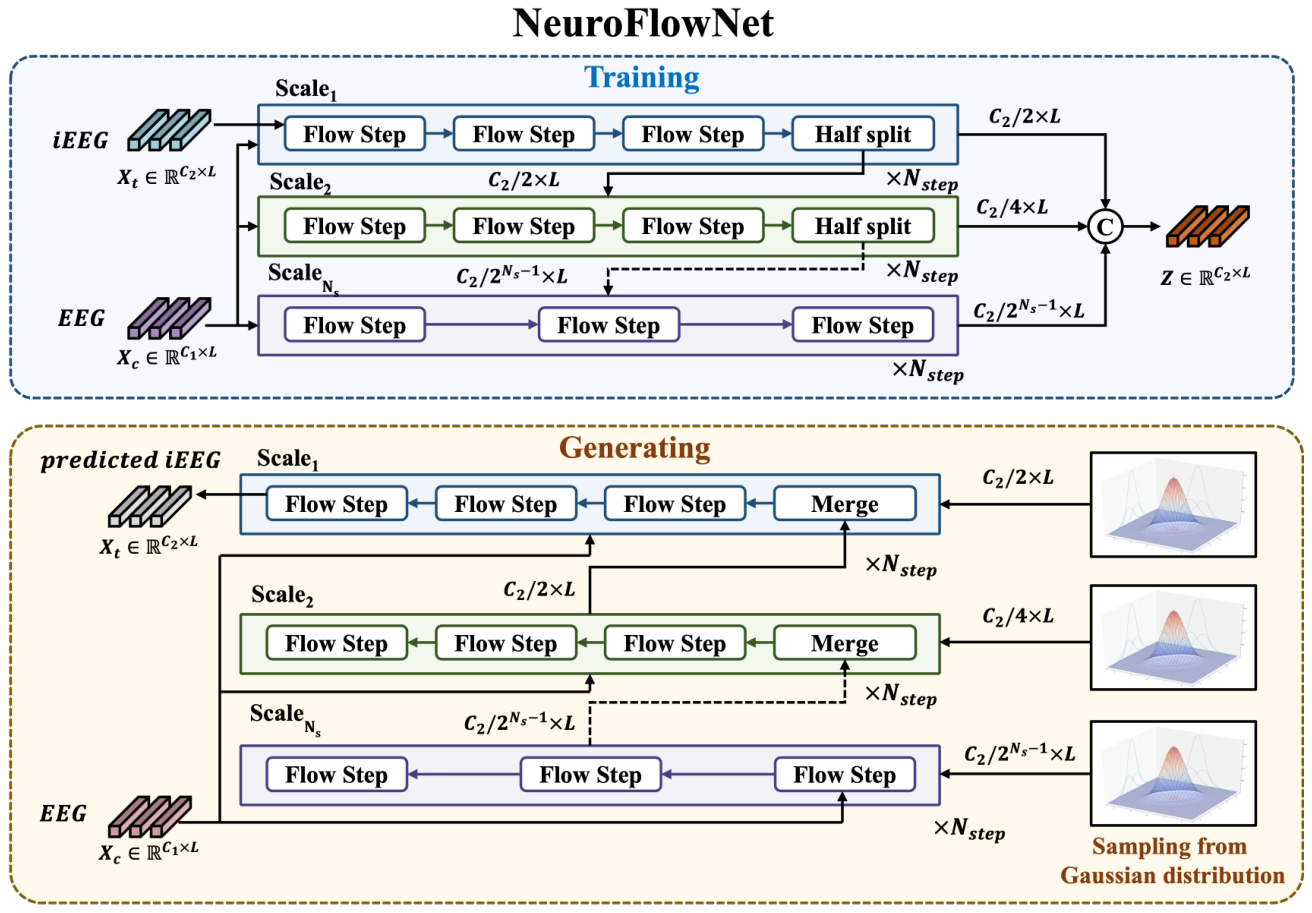
Figure 1. Figure 1: Overview of NeuroFlowNet architecture. The model consists of multiple scales, each containing a series of flow steps that transform the iEEG data conditioned on the EEG data. The final latent variable Z is obtained by concatenating the outputs from all scales.解説: NeuroFlowNetアーキテクチャの概要を示しています。モデルは複数のスケールで構成されており、各スケールは一連のフローステップを含んでいます。これらのフローステップは、EEGデータを条件としてiEEGデータを変換します。学習フェーズではiEEGデータから潜在変数Zを生成し、生成フェーズでは潜在変数ZとEEGデータからiEEGデータを生成する流れが示されています。
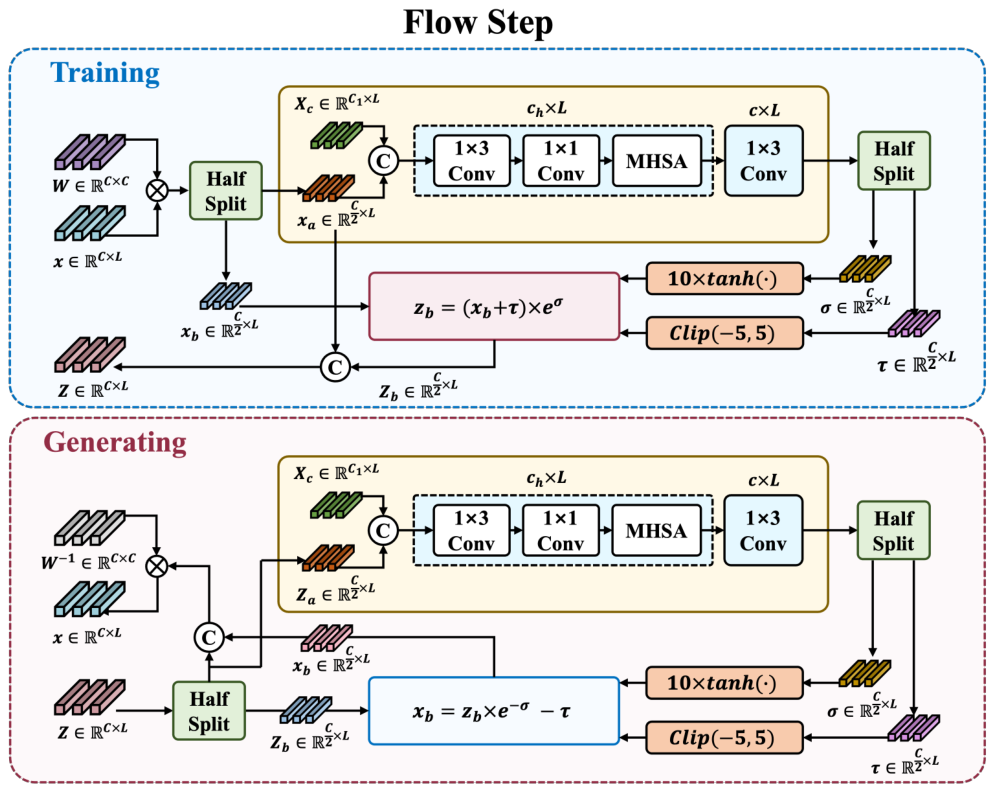
Figure 2. Figure 2: Flow step composition in NeuroFlowNet. Each flow step consists of an invertible 1 × 1 convolution followed by a conditional affine coupling layer, which transforms the input data while conditioning on the EEG data Xc.解説: NeuroFlowNetにおけるフローステップの構成を示しています。各フローステップは、可逆的な1×1畳み込み層と条件付きアフィンカップリング層で構成されており、EEGデータXcを条件として入力データを変換します。学習フェーズと生成フェーズのそれぞれにおけるデータの流れと変換プロセスが詳細に図示されています。
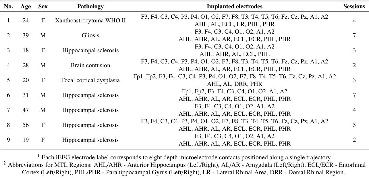
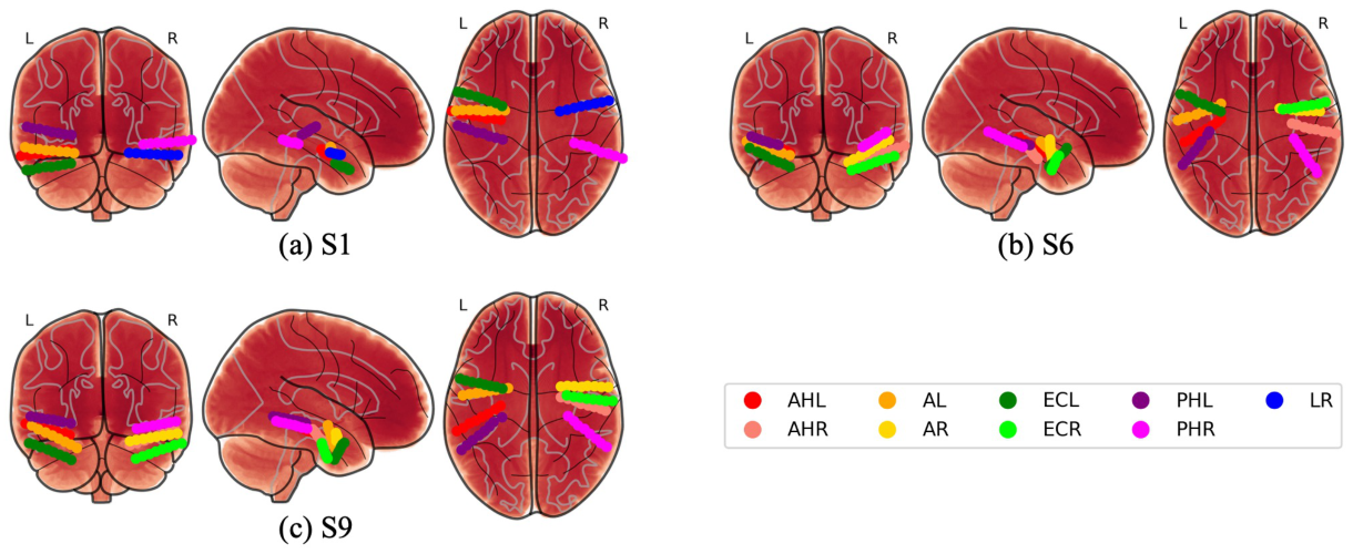
Figure 3. Figure 3: Medial temporal lobe (MTL) depth electrode locations for subjects used in this study (S1, S6 and S9). Each panel shows coronal, sagittal, and axial views of depth electrode trajectories within MTL subregions. Colors indicate anatomical targets: anterior hippocampus (AHL/AHR, red/light red), amygdala (AL/AR, orange/yellow), entorhinal cortex (ECL/ECR, green/light green), parahippocampal gyrus (PHL/PHR, pur- ple/magenta), and lateral rhinal area (LR, blue). Each trajectory consists of eight electrode contacts positioned along a single stereotactic path.解説: 本研究で使用された対象者(S1, S6, S9)の深部側頭葉(MTL)における深部電極の位置を3Dスキーマで示しています。各パネルは、MTLサブ領域内での深部電極の軌道の冠状、矢状、軸方向のビューを示しており、異なる色は前海馬、扁桃体、内嗅皮質、傍海馬回、側頭葉ライナル領域といった解剖学的ターゲットを示しています。
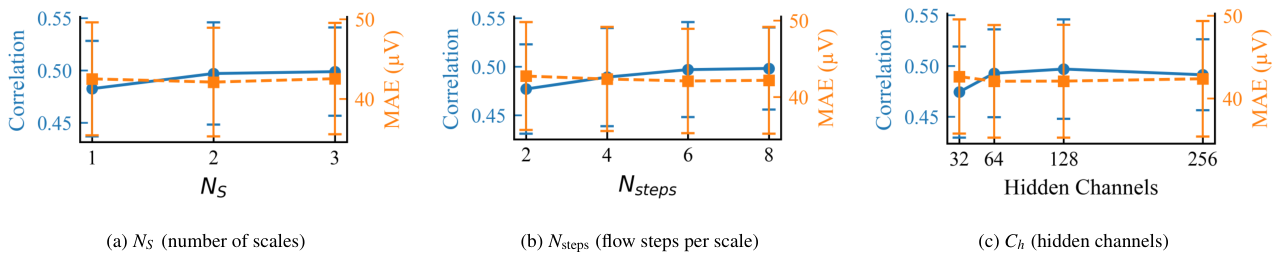
Figure 4. Figure 4: Hyperparameter selection results for NeuroFlowNet. The performance of the model is evaluated on the validation set and averaged across all subjects and electrodes. The hyperparameters include NS , the number of scales (a); Nsteps, the number of flow steps per scale (b); and Ch, the number of channels in the hidden layers of the conditional neural network (c). The results indicate that the model achieves optimal performance with NS = 2, Nsteps = 6, and Ch = 128.解説: NeuroFlowNetのハイパーパラメータ選択の結果を示しています。モデルの性能は検証セットで評価され、全ての対象者と電極で平均されています。ハイパーパラメータには、スケール数NS (a)、スケールあたりのフローステップ数Nsteps (b)、条件付きニューラルネットワークの隠れ層のチャネル数Ch (c) が含まれます。図はNS=2、Nsteps=6、Ch=128で最適な性能が得られることを示唆しています。
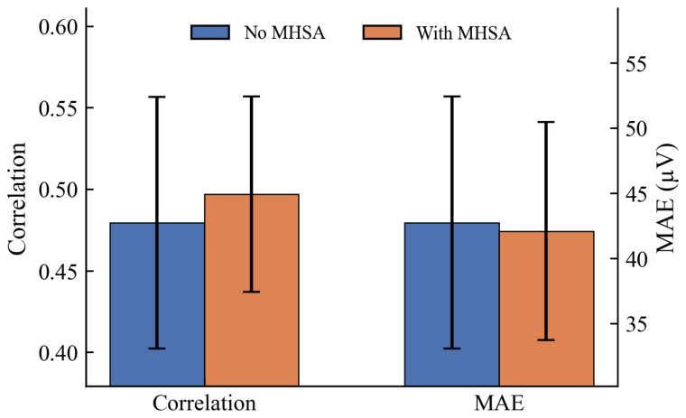
Figure 5. Figure 5: Ablation of the MHSA module in the conditional network gcond. Correlation (higher is better) and MAE (lower is better) are reported on the validation set. Bars indicate the mean across subjects and electrodes, and error bars denote the standard deviation across subjects解説: 条件付きネットワークgcondにおけるMHSA(マルチヘッド自己注意)モジュールのアブレーション(除去)研究の結果を示しています。検証セットにおける相関(高いほど良い)とMAE(低いほど良い)が報告されています。MHSAを組み込むことで、相関が向上し、MAEがわずかに減少することが示されています。
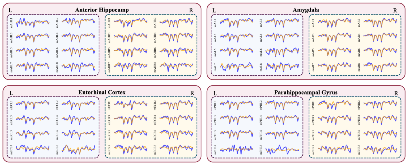
Figure 6. Figure 6: Exemplar generated iEEG signals (orange) overlaid with ground truth iEEG signals (blue) for various MTL subregions, specifically showing a 200ms segment from Subject S6. The figure illustrates the performance of NeuroFlowNet in generating iEEG signals from EEG data across different anatomical targets, including anterior hippocampus (AHL/AHR), amygdala (AL/AR), entorhinal cortex (ECL/ECR), and parahippocampal gyrus (PHL/PHR).解説: 対象者S6の様々なMTLサブ領域(前海馬、扁桃体、内嗅皮質、傍海馬回)について、生成されたiEEG信号(オレンジ色)と実際のiEEG信号(青色)を重ねて示す200msの代表的なセグメントです。NeuroFlowNetがEEGデータからiEEG信号を生成する性能を異なる解剖学的ターゲットにわたって視覚的に比較しています。
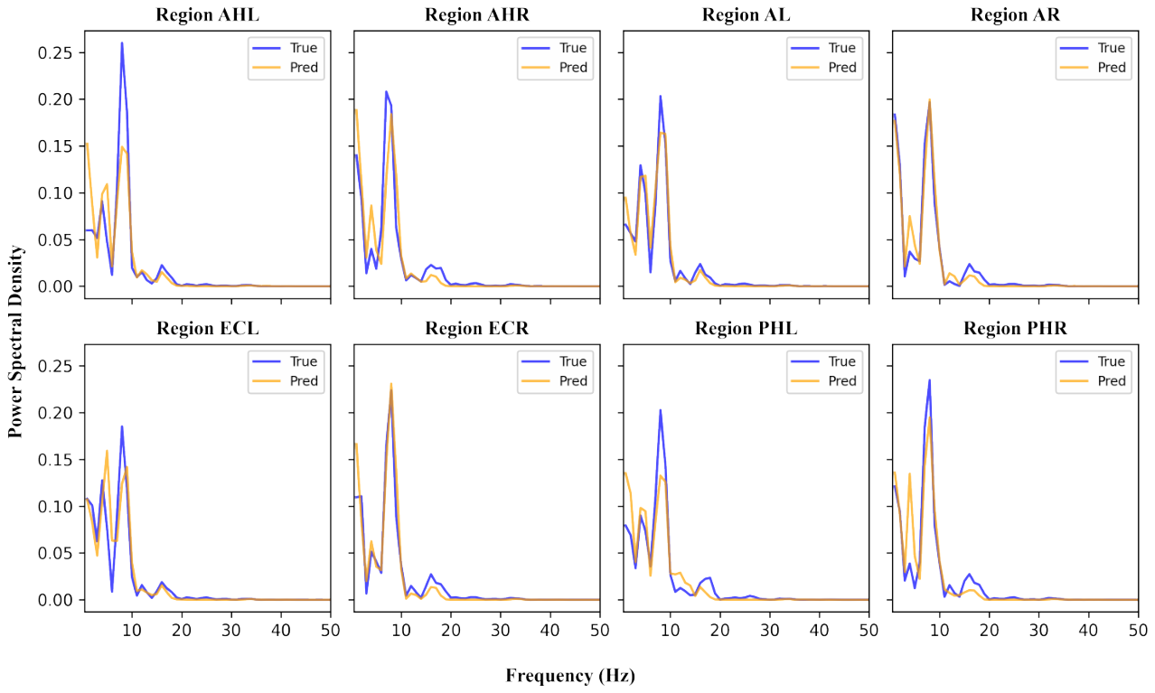
Figure 7. Figure 7: Comparison of power spectral density (PSD) between ground truth iEEG signals (blue) and generated iEEG signals (orange) for a 200 ms segment from Subject S6. The figure shows the average PSD across all electrodes within each MTL subregion, including anterior hippocampus (AHL/AHR), amygdala (AL/AR), entorhinal cortex (ECL/ECR), and parahippocampal gyrus (PHL/PHR).解説: 対象者S6の200msセグメントにおける、実際のiEEG信号(青色)と生成されたiEEG信号(オレンジ色)のパワースペクトル密度(PSD)の比較を示しています。図は、前海馬、扁桃体、内嗅皮質、傍海馬回を含む各MTLサブ領域内の全ての電極で平均されたPSDを示しており、モデルがスペクトル特性をよく再現していることを示しています。
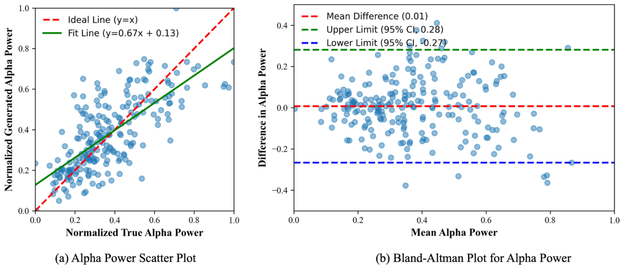
Figure 8. Figure 8: (a) Scatter plot of normalized true alpha power versus normalized generated alpha power. The red dashed line represents the ideal line (y = x), while the green solid line indicates the linear fit (y = 0.67x + 0.13). (b) Bland-Altman plot showing the difference in alpha power against the mean alpha power. The red dashed line indicates the mean difference (0.01), and the green and blue dashed lines represent the upper (95% CI, 0.28) and lower (95% CI, -0.27) limits of agreement, respectively.
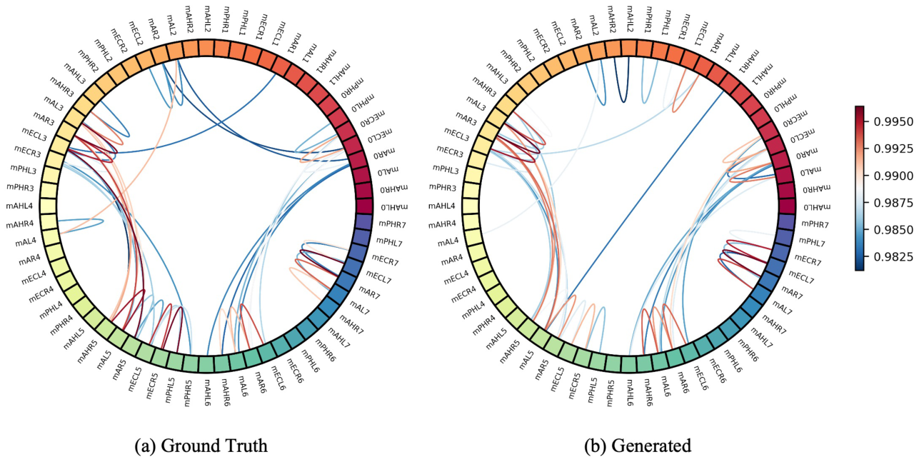
Figure 9. Figure 9: Comparison of inter-channel correlation. Circular graphs show the connectivity patterns of (a) the original iEEG signals and (b) the generated iEEG signals. Both plots illustrate a 200 ms segment from Subject S6. Pairwise Pearson correlation coefficients are computed between all channels, and only the top 50 strongest absolute correlations are visualized for clarity.
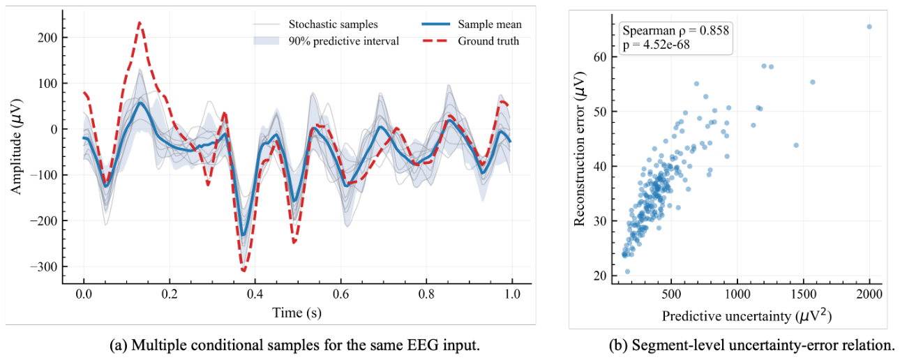
Figure 10. Figure 10: Representative conditional sampling and uncertainty analysis for Subject S6. (a) For a fixed scalp EEG segment, K = 20 independent latent samples generate multiple iEEG trajectories for channel mAHL1. The solid line denotes the sample mean, the shaded area denotes the empirical 90% predictive interval, and the dashed line denotes the ground-truth iEEG. (b) Across all validation segments of S6, each point represents one segment. Predictive uncertainty is defined as the mean sample variance across channels and time, and reconstruction error is defined as the MAE between the sample mean and the ground truth. Higher predictive uncertainty is strongly associated with larger reconstruction error (ρ = 0.858,

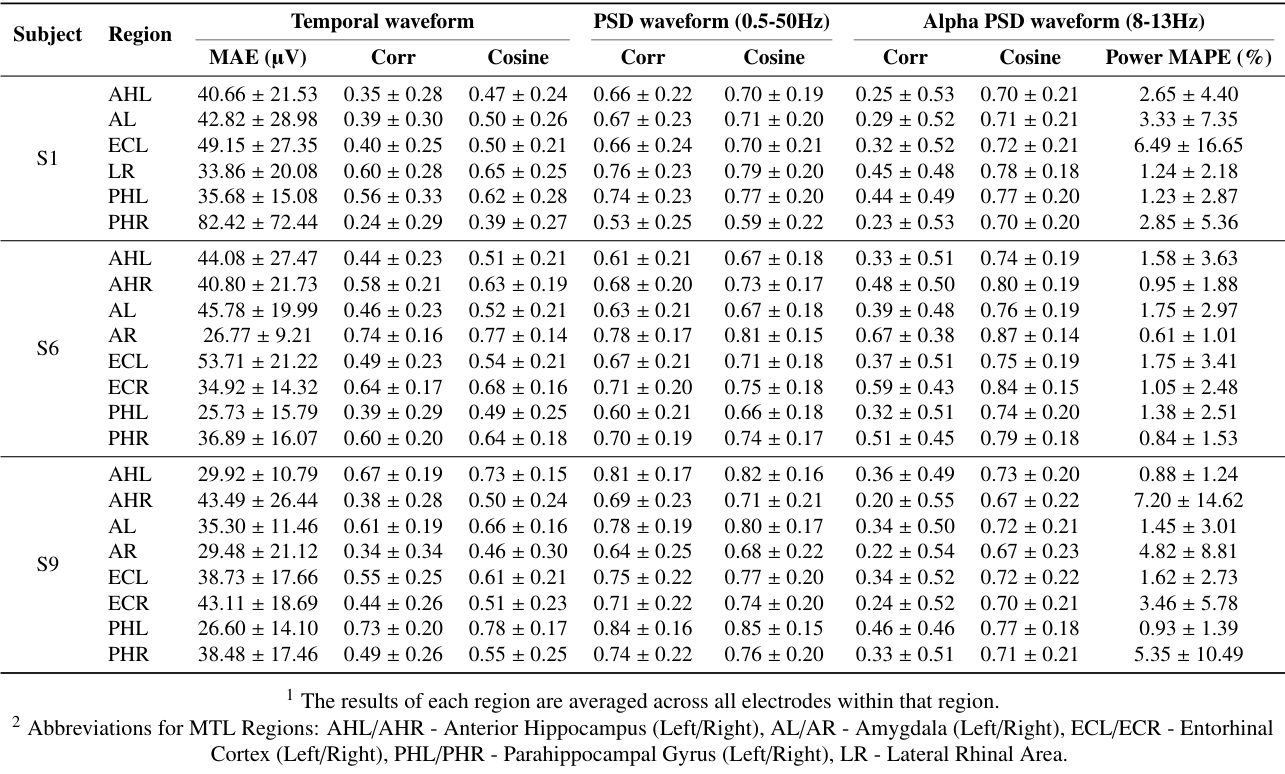
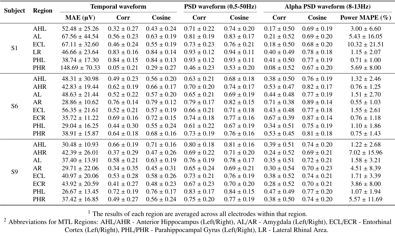

コメントを残す