どうも、Beyond the Pixelです。医療画像診断において、SPECT(単一光子放出コンピューター断層撮影)は、体内の放射性トレーサー分布を画像化する重要なモダリティです。このトレーサー分布を再構成する過程は、不完全でノイズのある投影データから元の情報を導き出すという、計算上困難な逆問題に直面します。従来の再構成手法は、単一の最適な画像推定値(ポイント推定)を生成しますが、この推定値にどれくらいの不確実性があるのか、また、その推定値が測定データとどれだけ適合しているのかを直接的に示すことはできませんでした。本研究論文は、「Physics in Medicine and Biology」に掲載された「Hamiltonian dynamics for stochastic reconstruction in emission tomography」というタイトルで、この課題に対する新たな確率論的フレームワークを提案しています。
2. ハミルトニアンモンテカルロ法(Hamiltonian Monte Carlo: HMC)によるサンプリング: SGDで特定された領域から、HMCを用いてデータと互換性のある画像アンサンブルを生成します。HMCは、古典力学の概念を利用して高次元空間を効率的に探索するマルコフ連鎖モンテカルロ法の一種です。これにより、再構成された画像における変動に関する統計的な情報を取得できます。
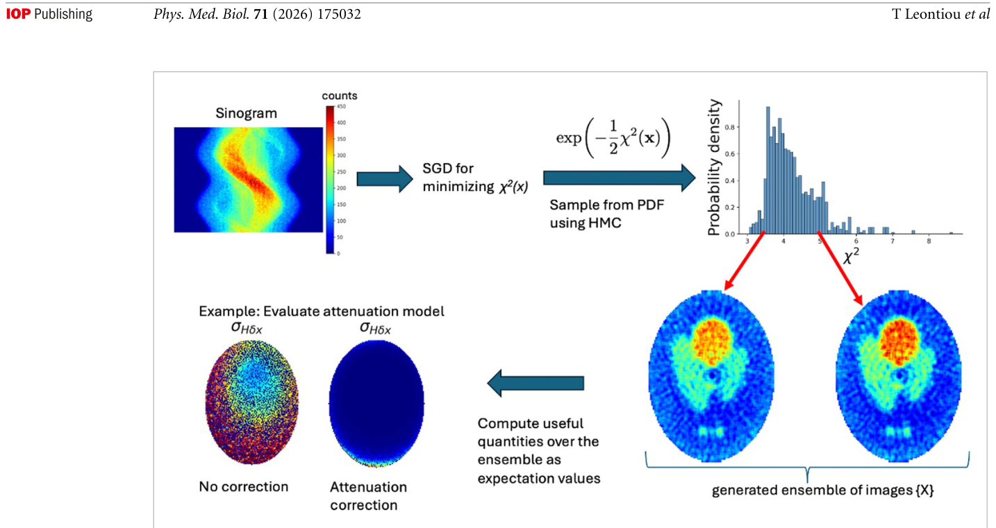
Figure 1. Figure 1. Overview of the stochastic reconstruction workflow and the concept of data-visible standard deviation. Starting from the measured detector sinogram (top left), a likelihood-based density over admissible images is defined as Π(x) ∝ exp[−χ2(x)/2] (top middle). A fast gradient-based reconstruction is first used to locate a high-probability region of this den- sity, providing initialization for Hamiltonian Monte Carlo sampling. HMC then generates an ensemble of reconstructed images; the top-right panel illustrates the resulting χ2 distribution, and the example images correspond to representative samples from the ensemble. From the generated ensemble, voxel-wise means, variances, and derived observables can be computed directly. The data-visible standard deviation is obtained by propagating ensemble fluctuations through the data-weighted projection– backprojection operator H = P⊤WP, thereby isolating the component of the sampled variability that remains coupled to the measured projection data. Comparison of these diagnostics under different forward-model assumptions, such as with and with- out AC, allows the ensemble to be used for assessing forward-model adequacy beyond global residual measures.解説: 確率論的再構成の全体的な流れとデータ可視標準偏差の概念を示しています。測定されたシノグラムから始まり、HMCサンプリングによってデータと互換性のある画像アンサンブルが生成され、そのアンサンブルから、減弱補正の有無によるデータ可視標準偏差の変化を比較する診断情報が得られることを視覚的に説明しています。
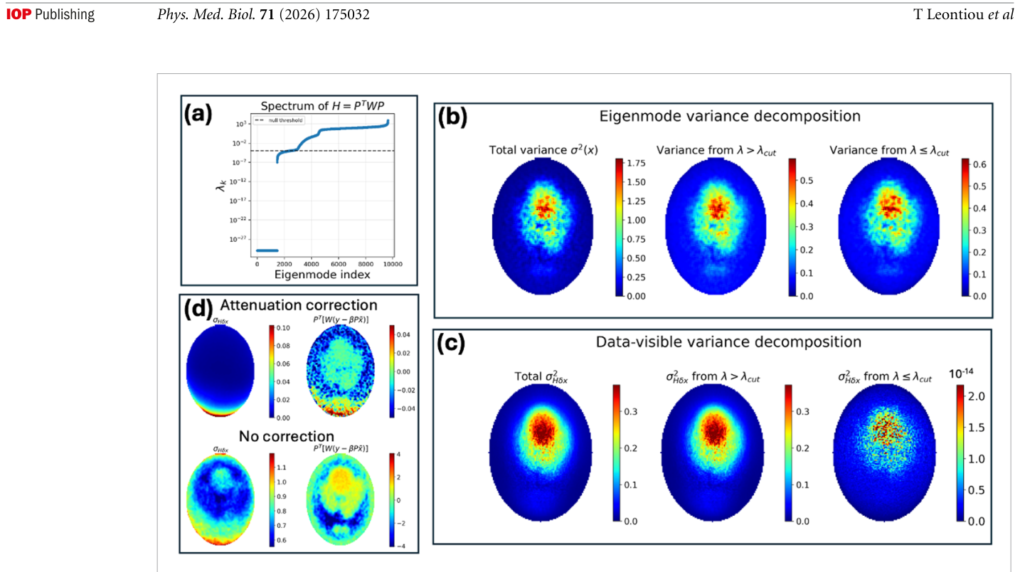
Figure 3. Figure 3. Data-visible variance, null/near-null-space decomposition, and comparison with the weighted residual backprojection. (a) Spectral analysis of H = P⊤WP in the masked image domain. The dashed line indicates the cutoff λcut used to distinguish weakly constrained modes from the remaining subspace. (b) Decomposition of the ordinary image variance. The total variance σ2(˜x) is separated into contributions from modes with λ > λcut and λ ⩽λcut. The low-eigenvalue modes contribute substan- tially to the ordinary image variance, showing that the sampled ensemble contains fluctuations in weakly constrained directions. (c) Decomposition of the data-visible standard deviation. The contribution from low-eigenvalue modes is strongly suppressed because Huk = λkuk. Thus, modes that contribute appreciably to ordinary image variance but are weakly coupled to the mea- sured projection data are largely removed from the data-visible variance. (d) Comparison between the data-visible standard deviation and the weighted residual backprojection P⊤W(y −βP˜x) for reconstructions with and without AC. The residual back- projection remains sensitive to structured mismatch in the ensemble mean, whereas the data-visible variance measures the scale of sampled fluctuations that remain coupled to the data. With AC, the data-visible variance is strongly reduced, while the residual structure is also reduced but not completely eliminated.解説: データ可視分散、ヌル空間/準ヌル空間分解、および重み付き残差逆投影との比較を示しています。(a) マスクされた画像ドメインにおけるH=P⊤WPのスペクトル分析、(b) 通常の画像分散の分解、(c) データ可視標準偏差の分解、(d) 減弱補正の有無によるデータ可視標準偏差と重み付き残差逆投影の比較を示し、両者が異なる再構成側面を測定することを示唆しています。
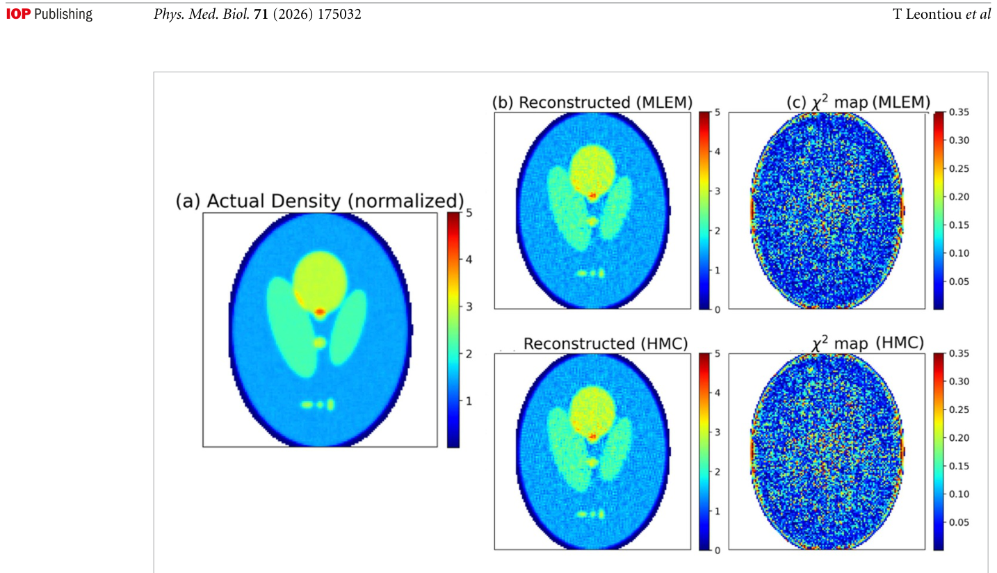
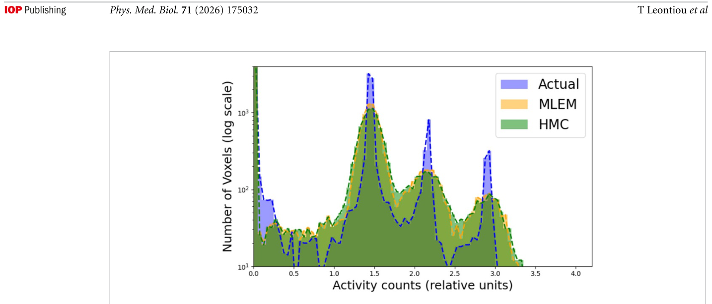
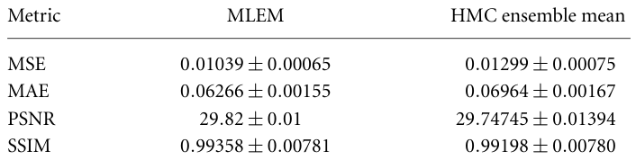
Figure 4. Figure 4. Idealized benchmark against deterministic reconstruction. (a) True activity distribution, normalized to the same scale as the reconstructions. The right panels show the MLEM reconstruction and local χ2 map, together with the HMC ensemble- mean reconstruction and its corresponding local χ2 map. This benchmark uses an effectively unphysical very-high-count acqui- sition and an ideal collimator assumption, and should therefore be interpreted as a limiting consistency test rather than as a realistic imaging scenario. The χ2 map metric is analyzed in detail in Frixou et al (2026).解説: 確定的再構成に対する理想的なベンチマーク評価を示しています。(a) 真の活動分布、(b) MLEMとHMCアンサンブル平均による再構成結果、(c) それらに対する局所的なχ²マップを比較し、HMCアンサンブル平均が理想的な条件下で確定的再構成と同等の精度を示すことを確認しています。Figure 5. Figure 5. Voxel-intensity histograms for the true image, MLEM reconstruction, and HMC ensemble mean. The comparison shows global agreement in the recovered intensity distribution under idealized high-count conditions. This metric is analyzed in detail in Frixou et al (2026).解説: 真の画像、MLEM再構成、およびHMCアンサンブル平均のボクセル強度ヒストグラムを比較しています。理想的な高カウント条件下で、回復された強度分布が全体的に一致していることを示しています。Table 1. Table 1. Reconstruction quality metrics for the idealized benchmark (mean ± standard deviation).
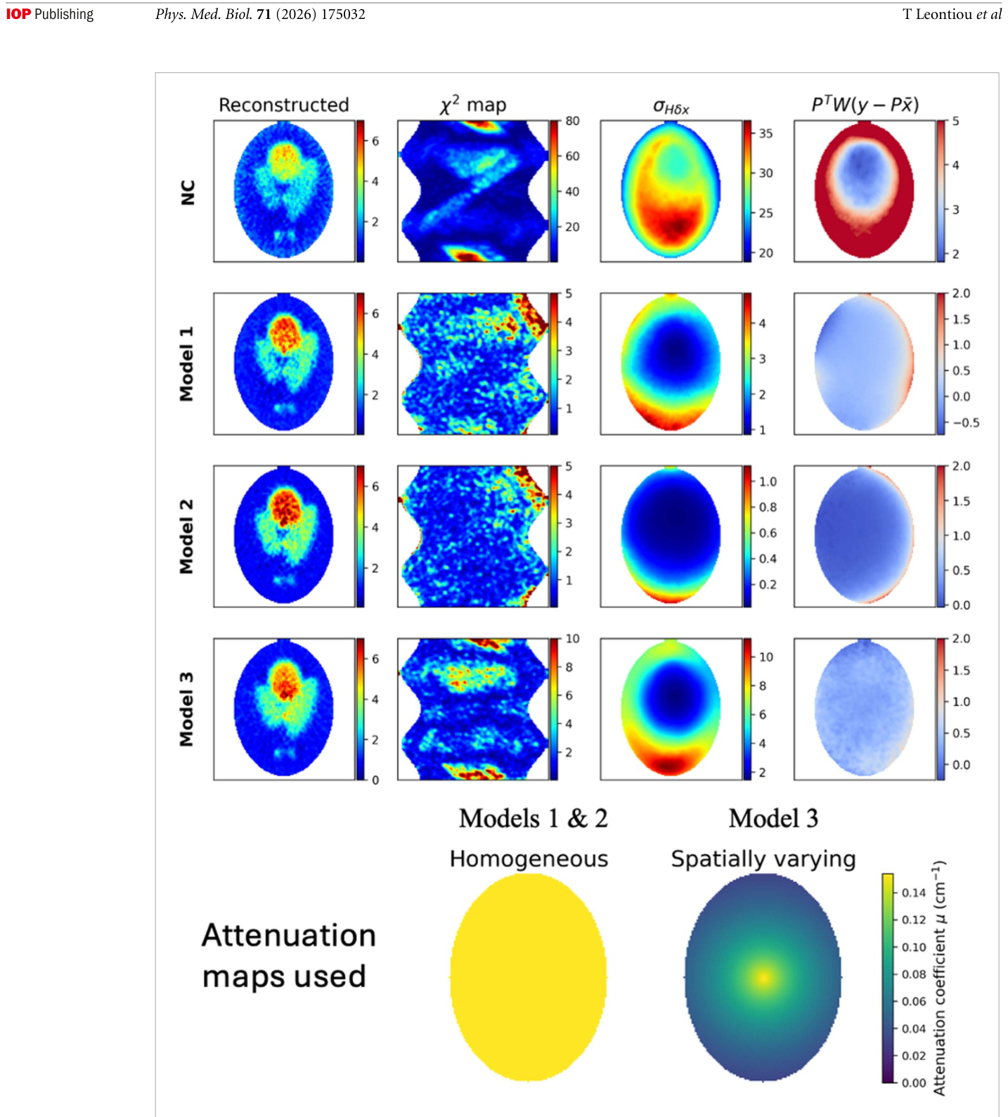
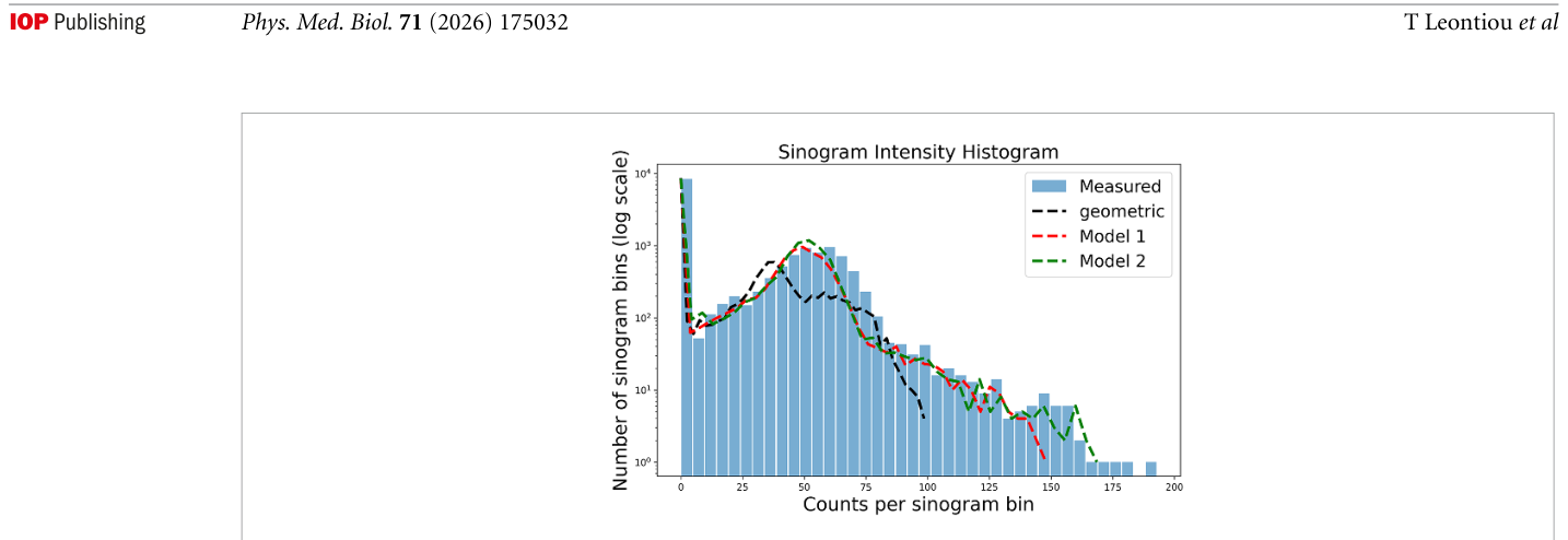
Figure 6. Figure 6. Application of the HMC framework to a realistic 3D voxelized software phantom. The upper rows show, for each forward-model configuration, the ensemble-mean reconstruction, the spatially resolved χ2 map, the sampled data-visible standard deviation σHδx, and the weighted residual backprojection PTW(y −Px). Rows correspond to NC, Model 1, Model 2, and Model 3. The bottom row shows the attenuation coefficient maps used in the attenuation models: a homogeneous water- equivalent map and a spatially varying map, both displayed with a common colorbar in units of cm−1.解説: 現実的な3Dボクセル化ソフトウェアファントムへのHMCフレームワークの適用結果を示しています。減弱補正なし(NC)、均一減弱補正(Model 1)、現実的なコリメータモデルと組み合わせた減弱補正(Model 2)、不完全な減弱補正(Model 3)の各フォワードモデル設定に対して、再構成画像、χ²マップ、サンプリングされたデータ可視標準偏差、および重み付き残差逆投影を比較しています。下段には各減弱マップも示されています。Figure 7. Figure 7. Sinogram intensity histograms comparing measured projection data with projections predicted by different forward models. The purely geometric model (black dashed line) shows substantial discrepancy with the measured data. Introducing AC using a homogeneous water-equivalent medium in GATE (red dashed line, Model 1) improves agreement across a broad range of count levels. Further refinement is observed when a non-uniform attenuation model derived from the experimental attenuation map is used (green dashed line, Model 2). While these histograms demonstrate progressive global improvement, they do not reveal the spatial origin of the remaining discrepancies.解説: 異なるフォワードモデルによって予測された投影データと、測定された投影データを比較するシノグラム強度ヒストグラムを示しています。測定データと幾何学的モデル、Model 1、Model 2の予測を比較し、モデルの改善が測定データとの整合性を向上させる様子を示唆しています。
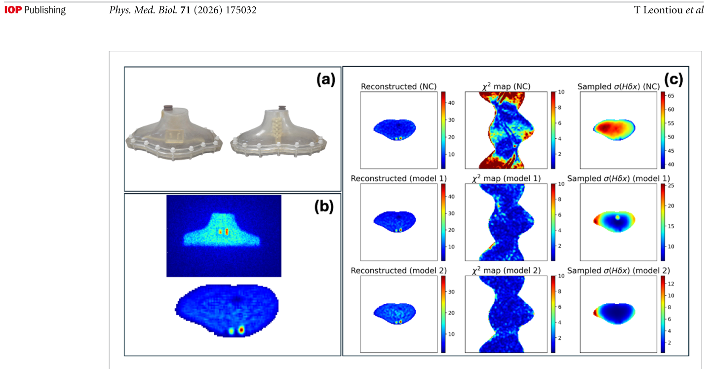
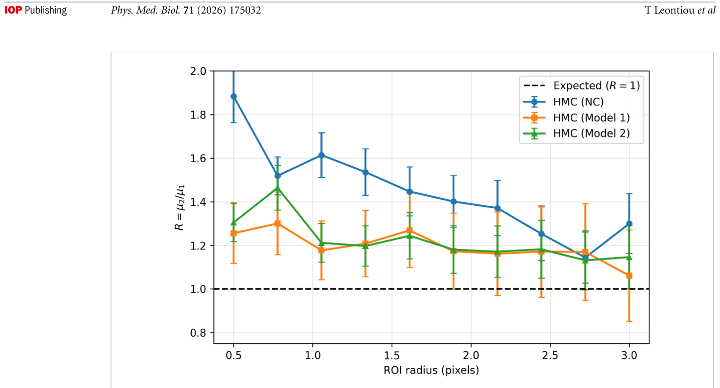
Figure 8. Figure 8. Application of the HMC framework to the thyroid phantom experiment. Panel (a) shows photographs of the exper- imental thyroid phantom. Panel (b) displays a representative detector projection (top) and the corresponding reconstructed central slice (bottom) used for the analysis. Panel (c) presents the reconstruction analysis. Each row corresponds to a different forward model. Left column: reconstructed central slice (ensemble mean). Middle column: spatially resolved χ2 map comparing measured and predicted sinograms. Right column: sampled data-visible deviation σHδx. Top row (NC): geometric projection model without AC. Second row (Model 1): GATE-based simulation using a homogeneous water-equivalent attenuation model and collimator response. Third row (Model 2): macroscopic non-uniform attenuation model with spatially varying attenuation coefficients optimized from the experimental data. While global χ2 decreases with progressive model refinement, the χ2 maps become increasingly noise-like, limiting their spatial diagnostic value. In contrast, the sampled σHδx maps provide a clearer indi- cation of how image fluctuations project into data-sensitive directions. The non-uniform attenuation model produces a marked suppression of σHδx near object boundaries, demonstrating that forward-model improvements primarily affect regions where attenuation heterogeneity is most significant, while the bulk variability remains largely governed by intrinsic ill-posedness and counting statistics. The σHδx maps are shown normalized by the mean reconstructed activity within the object mask (dimension- less, relative to image mean).解説: 甲状腺ファントム実験へのHMCフレームワークの適用結果を示しています。(a) 実験用ファントムの写真、(b) 真の活動分布、(c) 減弱補正なし(NC)、Model 1、Model 2の各フォワードモデル設定での再構成画像、χ²マップ、サンプリングされたデータ可視標準偏差を比較しています。Figure 9. Figure 9. Ensemble-based quantitative assessment from the thyroid phantom. For each ROI radius r, the lesion-to-lesion mean- intensity ratio R(r) = µ2(r)/µ1(r) was computed sample-wise from the HMC ensemble using variance-weighted ROI means (equation (31)) and summarized by the mean and standard deviation (equation (33)). Error bars represent the standard devia- tion of R(r). The dashed line indicates the expected concentration ratio Rtrue = 1. The plateau behavior demonstrates robustness with respect to ROI radius, while convergence toward Rtrue and reduced inter-model spread with improved attenuation modeling indicate enhanced quantitative consistency. This example illustrates how ensemble-based reconstruction enables estimation of derived observables together with ensemble-derived uncertainty estimates under the adopted sampling model.解説: 甲状腺ファントムからのアンサンブルベースの定量的評価を示しています。各ROI(関心領域)半径 r について、病変対病変の比率のHMC推定値(NC、Model 1、Model 2)と期待値(R=1)を比較し、モデルの改善が定量値の不確実性を減少させ、期待値に近づけることを示しています。
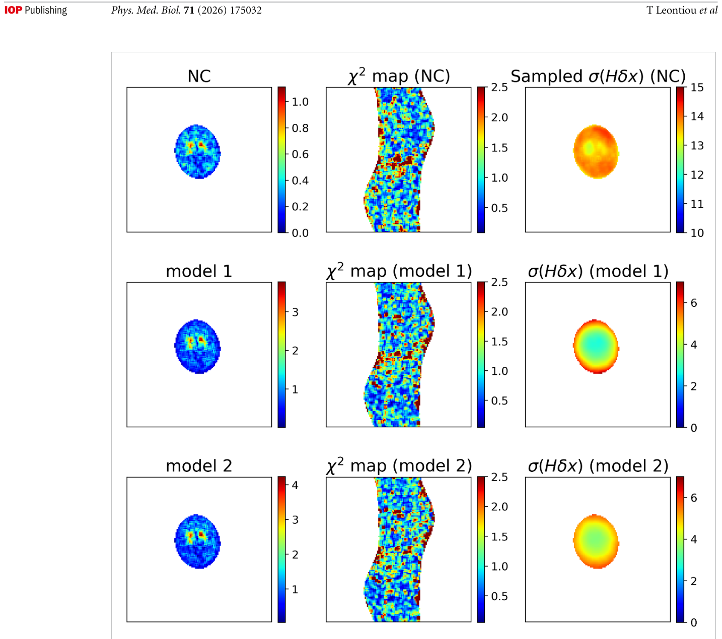
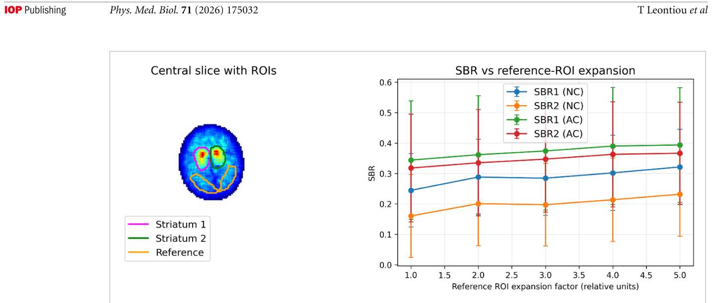
Figure 10. Figure 10. Application of the HMC framework to a clinical DATSCAN SPECT study. Each row corresponds to a different forward-model configuration. Left column: reconstructed central slice (ensemble mean). Middle column: spatially resolved χ2 map comparing measured and predicted sinograms. Right column: sampled data-visible standard deviation σHδx. Top row (NC): geometric projection without AC. Middle row (Model 1): homogeneous water-equivalent attenuation model. Bottom row (Model 2): homogeneous water-equivalent attenuation model augmented with a skull component. While the χ2 maps exhibit largely noise-like residual structure with limited distinction between models, the σHδx maps provide a clearer spatial diagnostic of variability. The absence of systematic suppression of σHδx across these attenuation refinements suggests that further improve- ment requires investigation of additional forward-model components beyond simple homogeneous attenuation modeling. The higher overall magnitude of σHδx compared with the controlled phantom studies reflects the absence of patient-specific attenua- tion information and the increased modeling uncertainty inherent to clinical data.解説: 臨床DATSCAN SPECT研究へのHMCフレームワークの適用結果を示しています。各行は異なるフォワードモデル設定(NC、Model 1、Model 2)に対応し、中央再構成画像、χ²マップ、サンプリングされたデータ可視標準偏差を比較しています。Figure 11. Figure 11. Quantitative striatal binding ratio (SBR) analysis for the clinical DATSCAN study. Left: central reconstructed slice (ensemble mean) with manually defined regions of interest (ROIs). The two upper ROIs correspond to the left and right striatal uptake regions, while the lower posterior ROI defines the reference region used for SBR normalization. Right: SBR estimates as a function of the fractional expansion of the reference ROI used to test robustness with respect to ROI definition. For each configuration, SBR values are computed sample-wise from the HMC ensemble according to equation (35), and the error bars represent the standard deviation across the sampled images. Results are shown for reconstructions without AC (NC) and with homogeneous (AC). While the absolute SBR values depend moderately on the reference ROI size, the estimates remain relatively stable across a broad range of expansion factors. The substantial uncertainty bars reflect the low-count clinical acquisition and the absence of patient-specific attenuation information. This example illustrates how ensemble-based reconstruction enables reporting clinically relevant uptake ratios together with uncertainty estimates derived directly from the sampled image ensemble.解説: 臨床DATSCAN研究における線条体結合比(SBR)の定量的分析を示しています。左図はROIが設定された中央スライスを示し、右図は参照ROIの拡張率に対するSBRの値を、減弱補正なし(NC)と減弱補正あり(AC)の場合について比較しています。SBRの不確実性とモデルへの依存性を示しています。
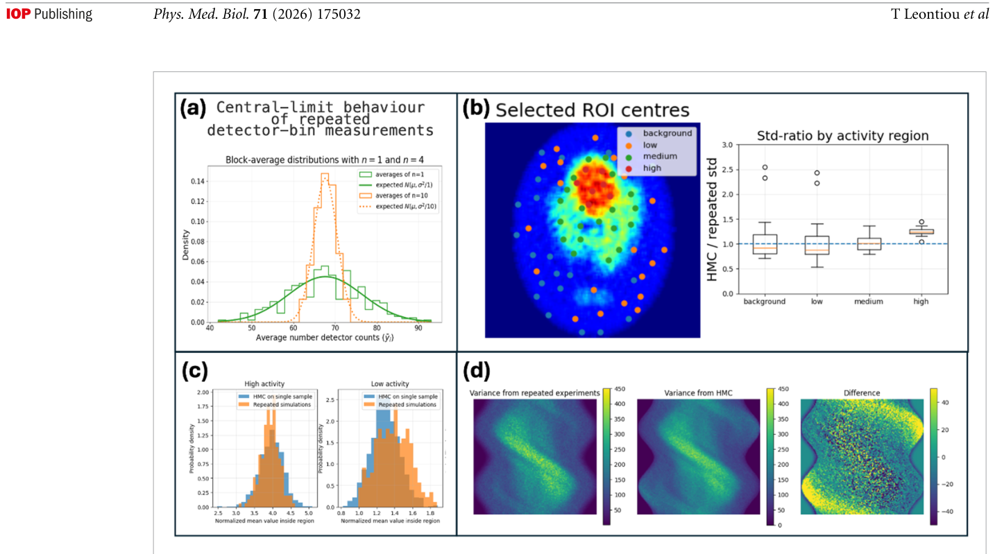
Figure 2. Figure 2. Empirical validation of the image ensemble generated from the likelihood-based compatibility density. (a) Central- limit behavior of repeated detector-bin measurements. Independent simulations of the same object were grouped into blocks, and the block-average count distributions were compared with the corresponding Gaussian approximations. This test supports the Gaussian weighted least-squares compatibility factor used in equation (4) for the count regime considered here. (b) Regional image-domain comparison. Circular regions were selected across background, low-, medium-, and high-activity parts of the reconstructed image. The radius of each region was chosen from the effective point-spread-function radius of the reconstruction pipeline, so that the comparison is performed at the spatial scale of the reconstructed resolution rather than at the level of indi- vidual voxels. For each region, the standard deviation of the normalized regional density ρR estimated from the sampled image ensemble was divided by the corresponding value obtained from repeated independent simulations followed by reconstruction. Values close to unity indicate good agreement in the predicted regional variability. (c) Representative distributions of ρR for high- and low-activity regions, comparing the sampled ensemble from a representative acquisition with the ensemble obtained from repeated simulations. (d) Projection-space validation. The standard deviation estimated from repeated simulated sinogram realizations is compared with the corresponding projection-space prediction obtained by forward projection of the sampled image ensemble. The difference image shows the residual between the two estimates. Further details of the simulations are given in section 3.4, and HMC implementation details are provided in appendix.解説: 尤度ベースの互換性密度から生成された画像アンサンブルの経験的検証結果を示しています。(a) 繰り返された検出器ビン測定における中心極限定理の挙動、(b) 画像ドメインでの領域比較、(c) 高活動および低活動領域における正規化された領域密度の分布比較、(d) 投影空間での標準偏差の比較を通じて、提案手法が統計的に整合性を持つことを確認しています。
Figure 12
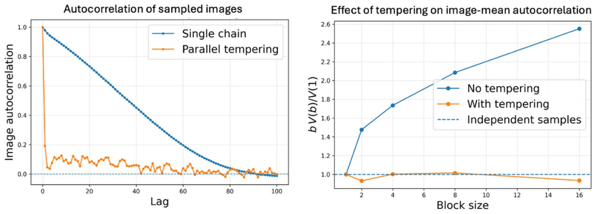
Figure 12. Figure 12. Effect of parallel tempering on HMC mixing. Left: image-level autocorrelation as a function of lag for a single HMC chain and for the parallel-tempered run. Right: blocking analysis for an image-mean observable. For independent samples, bV(b)/V(1) is expected to remain close to unity. Parallel tempering substantially reduces serial correlation and improves effec- tive sampling of the target-temperature ensemble.

コメントを残す