どうも、Beyond the Pixelです。MRIは、その優れた軟部組織の分類・特性評価能力により、診断医療において強力なツールとして広く活用されています。近年、7テスラMRI({{GLOSSARY_7T_MRI}})のような超高磁場システムと、ケミカル交換飽和移動({{GLOSSARY_CEST}})、定量的磁化率マッピング({{GLOSSARY_QSM}})、q空間軌道イメージング({{GLOSSARY_QTI}})、そしてナトリウム({{GLOSSARY_23Na_imaging}})イメージングといった先進的な定量的MRI技術の発展は、脳組織のさらなる微細な特性評価を可能にしつつあります。これらの技術は、従来の画像診断では捉えきれなかった、生体分子情報、鉄沈着、ミエリン含有量、イオン恒常性、細胞の生存度といった、より深い生物学的情報({{GLOSSARY_biosignature}})を引き出す可能性を秘めています。このアプローチは、個々のボクセル({{GLOSSARY_voxel}})から多様なMR特徴ベクトルを導出し、解剖学的情報に頼らず組織を分類する「ボクセロミクス({{GLOSSARY_voxelomics}})」と呼ばれ、将来の脳組織分類に革新をもたらすと考えられています。しかし、このように多くの先進的なコントラストを組み合わせるマルチパラメトリックMRI({{GLOSSARY_multiparametric_MRI}})プロトコルは、取得から後処理までのプロセスが複雑になり、新たな変動要因が生じることが懸念されます。信頼性の高いイメージングバイオマーカー、縦断的研究、そして機械学習の応用には、測定されたパラメータの再現性({{GLOSSARY_repeatability}})が不可欠です。本研究では、脳組織のボクセルごとの特性評価を目的とした拡張マルチパラメトリック7テスラMRIプロトコルの再現性を体系的に評価しました。
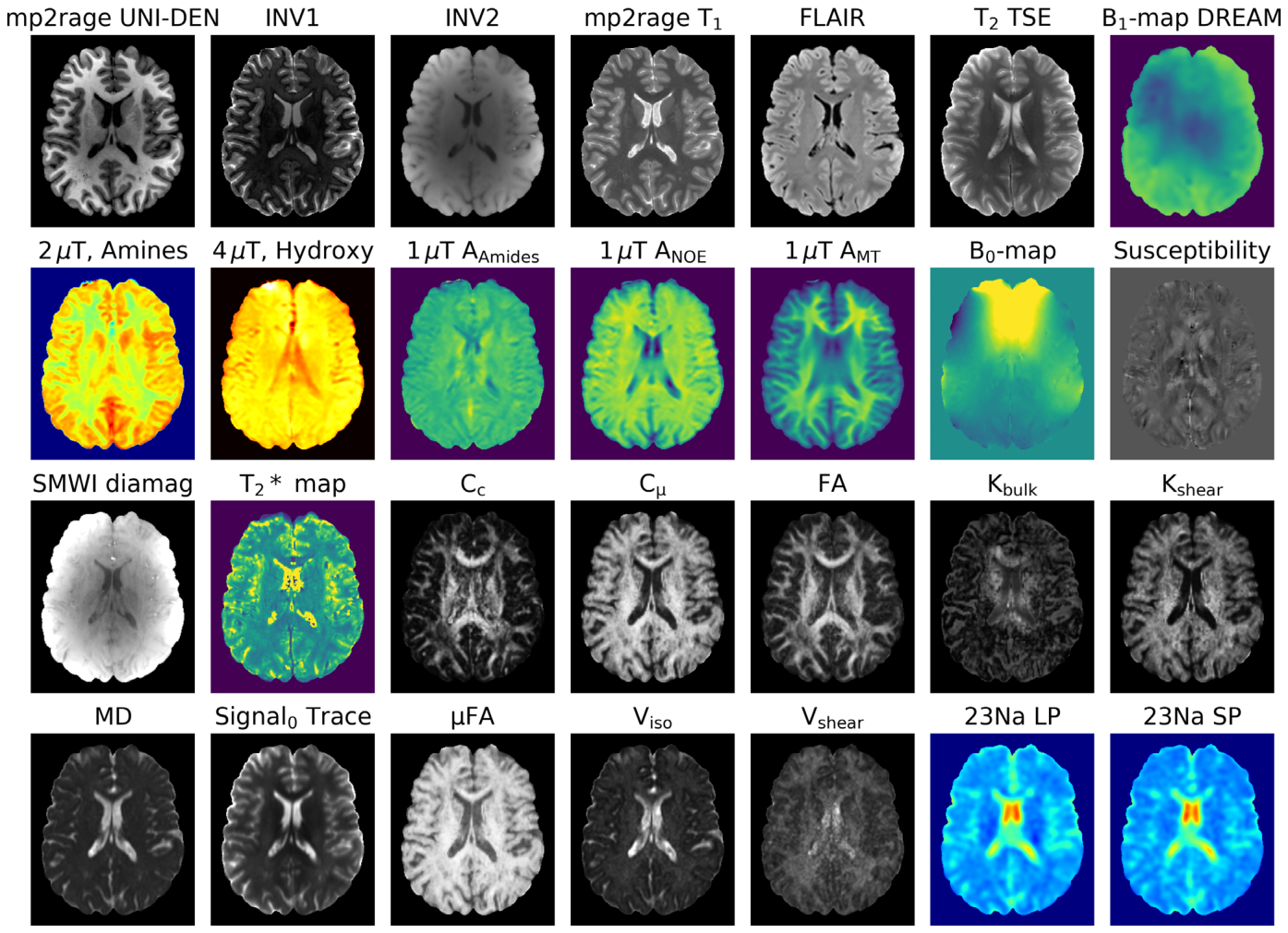
Figure 1. FIGURE 1 | Single slice of one imaging session for a subject showing 28 of 45 acquired MRI contrasts. The first set of images was obtained using product sequences of the vendor and provides anatomical reference. The following images depict various chemical exchange saturation transfer (CEST) contrasts. Subsequently, a susceptibility map and related contrasts using the data obtained from the same GRE sequence are shown. The next group of images presents diffusion-related information acquired using QTI. Finally, two images illustrate sodium within the brain.解説: 一つの撮像セッションで得られた、対象者の一枚の脳スライスにおける28種類のMRIコントラスト画像です。上段から形態学的画像、CESTコントラスト、磁化率マップ、QTI画像、ナトリウム画像が示されています。
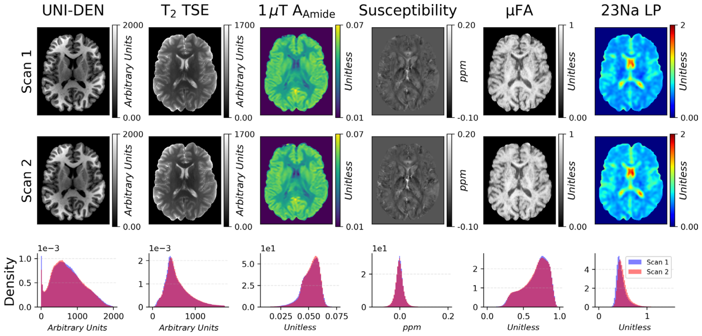
に示します。スキャン間での代表的なコントラストマップの比較と、それらの信号強度のヒストグラムを
Figure 2. FIGURE 2 | Visual comparison of representative contrast maps. Row 1: First scan: T1- and T2-weighted morphological images, CEST image, sus- ceptibility map, QTI—𝜇FA map, Sodium raw image. Row 2: Second scan. Row 3: Histograms of signal intensity over the entire brain volume of first and second scan.解説: 代表的なコントラストマップの視覚的比較です。上段は1回目のスキャン、中断は2回目のスキャン画像を示し、下段は各コントラストの全脳ボリュームにおけるボクセル強度ヒストグラムを示します。ほとんどのコントラストで両セッションの強度分布が高い一致度を示しています。
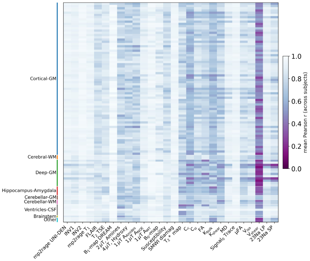
Figure 8. FIGURE 8 | Voxel-wise intra-subject correlation across the multi-parametric quantitative MRI protocol. For each subject, region, and contrasts, a Pearson correlation coefficient (r) was computed between voxel-wise intensity values of Scan 1 and Scan 2. Each cell shows this r-value averaged across all 12 subjects, for a given contrast (columns) and a given anatomical region (rows). Higher values (light) indicate strong voxel-wise linear agreement between repeated scans; lower values (dark) indicate weaker voxel-wise agreement between scans. Rows are grouped and color-coded by anatomical class along the left-hand axis (Cortical-GM, Cerebral-WM, Deep-GM, Hippocampus-Amygdala, Cerebellar-GM, Cerebellar-WM, Ventricles-CSF, Brain- stem, Other), with individual rows corresponding to regions within each class. The large majority of region-contrast combinations show high correlation (r < 0.6, light shading). Exceptions are concentrated in specific combinations rather than being widespread: Vshear and 23NA show reduced correlation particularly within Deep-GM structures.解説: マルチパラメトリック定量MRIプロトコルにおける、ボクセルごとの対象者内相関(ピアソン相関係数r)を示すヒートマップです。各セルは、指定されたコントラストと解剖学的領域における12名の対象者全体の平均r値を示します。値が高いほど、繰り返しスキャン間のボクセルごとの線形一致度が強いことを意味します。
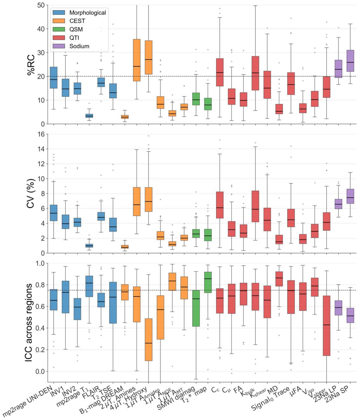
Figure 3. FIGURE 3 | Region-wise reliability metrics (%RC, CV (%), ICC) across the multiparametric MRI protocol. For each contrast, boxplots summarize the distribution of values across all segmented brain regions, with each data point representing one anatomical region (median: Horizontal line; box: Interquartile range; outliers: Gray dots). Contrasts are grouped and color-coded by contrast family (morphological, CEST, QSM, QTI, 23Na). Dashed horizontal lines indicate a reference threshold (%RC = 20%, ICC = 0.75). B0 and susceptibility were excluded, since they show consistently high CV and %RC in all regions of the brain, as a consequence of their value range centered around zero, which makes ratio-based metric unsuitable.解説: マルチパラメトリックMRIプロトコルにおける、各コントラストの領域ごとの信頼性指標(%RC、CV、ICC)を箱ひげ図でまとめたものです。コントラストは種類別に色分けされており、点線はそれぞれの参照閾値を示します。
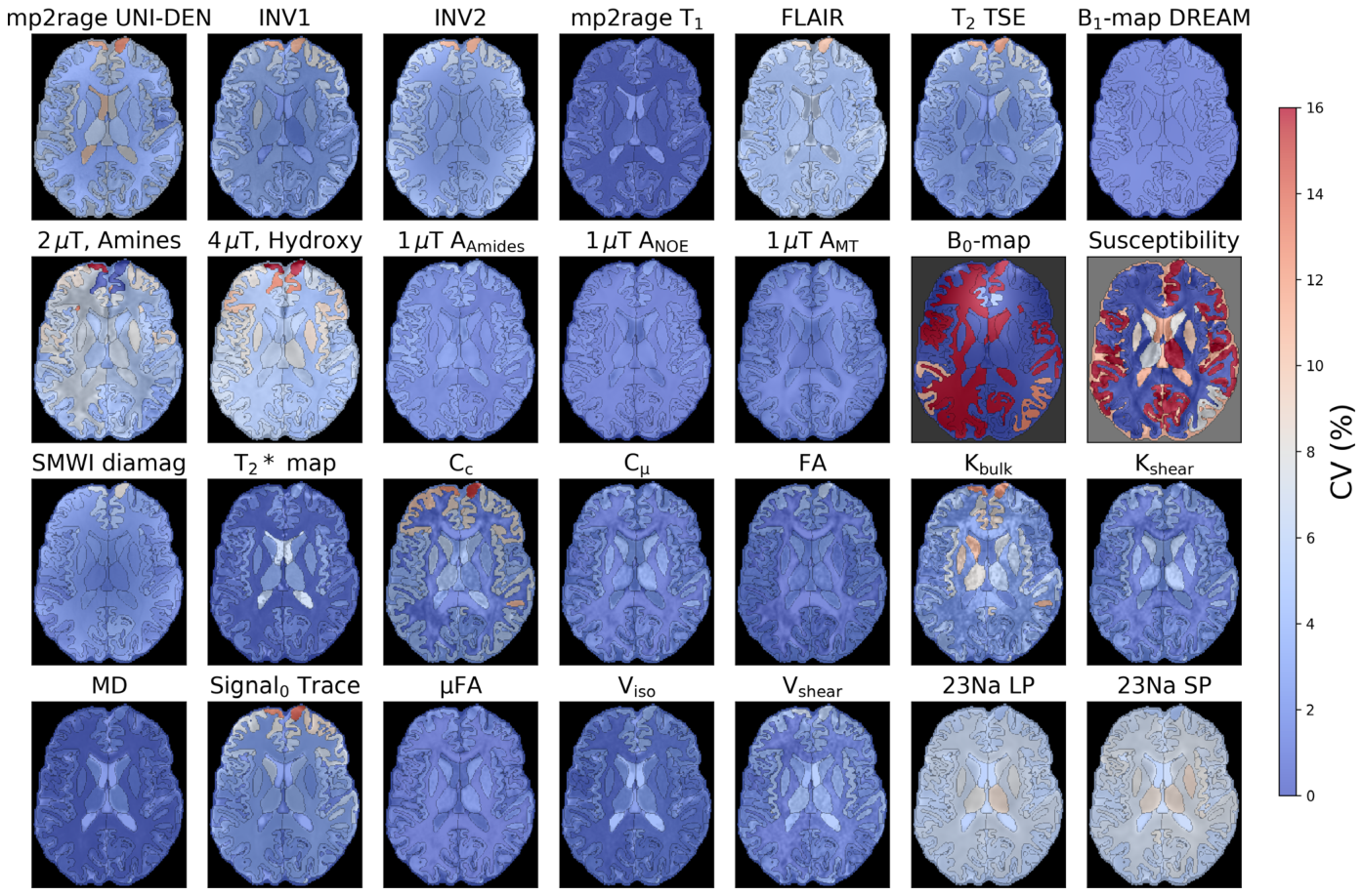
に、脳組織全体でのCVマップを
Figure 4. FIGURE 4 | Region-wise reproducibility (CV (%)) across a multiparametric quantitative MRI protocol. Axial CV maps (0%–16%) are shown for each of the quantitative contrasts, including morphologic imaging, CEST, QSM, QTI, and 23Na imaging. Most parameters show low CV (< 4%) throughout brain tissue, whereas B0 and susceptibility maps show elevated CV. This is due to their signed values being frequently close to zero.解説: マルチパラメトリック定量MRIプロトコルにおける、脳組織全体での領域ごとの再現性(CV%)マップです。ほとんどのパラメータで脳組織全体に低いCV(4%未満)が示されています。
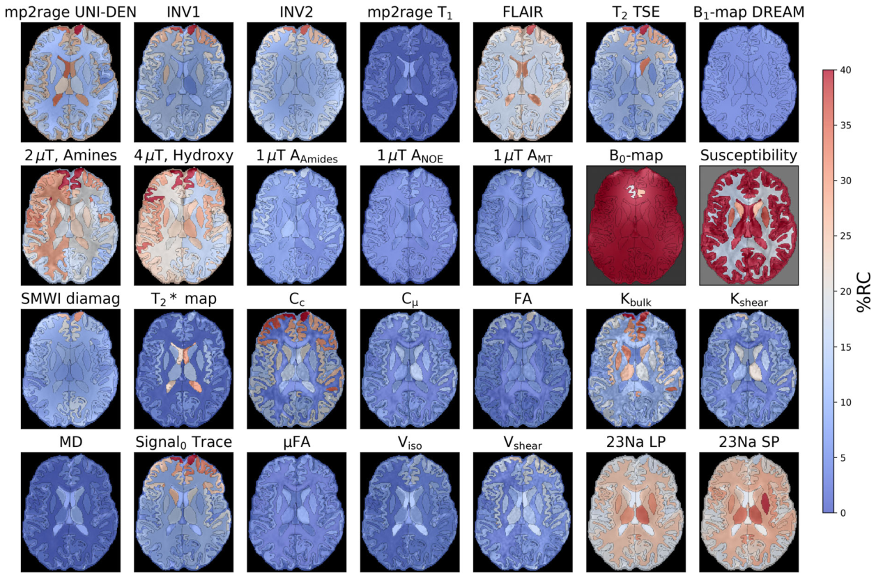
に、%RCマップを
Figure 5. FIGURE 5 | Region-wise repeatability (%RC) across a multiparametric quantitative MRI protocol. As a complementary reliability metric to the CV maps, %RC (0%–40%) for all quantitative contrasts. Most parameters again show low %RC (< 15%) across brain tissue, while Kbulk and 23Na metric show moderately elevated %RC in periventricular and deep gray matter regions B0 and susceptibility maps show near-saturated %RC values throughout as it is an unsuitable metric for the contrasts value range.解説: マルチパラメトリック定量MRIプロトコルにおける、脳組織全体での領域ごとの繰り返し測定可能性(%RC)マップです。CVマップと同様に、ほとんどのパラメータで低い%RC(15%未満)が脳組織全体で示されています。
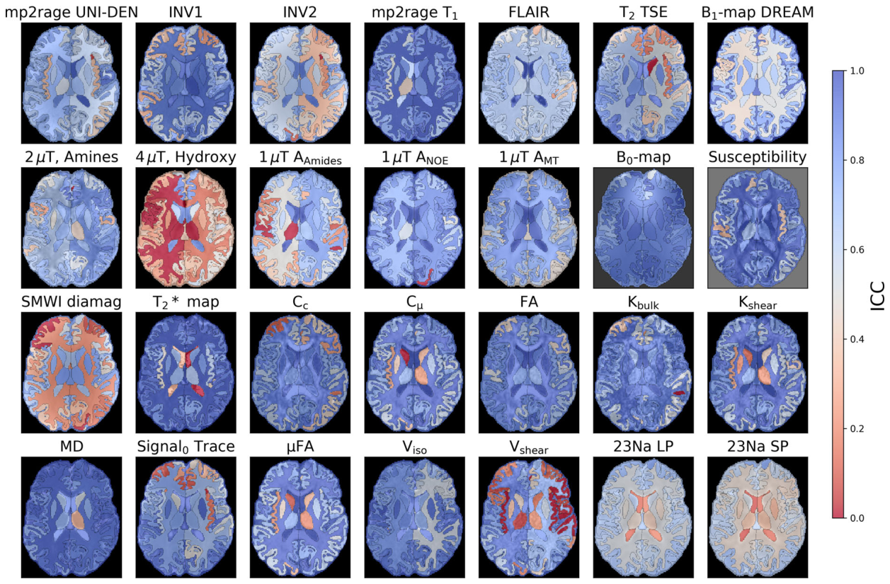
に、ICCマップを
Figure 6. FIGURE 6 | Region-wise ICC maps across the same multiparametric MRI protocol. ICC (0–1) provides a third, complementary measure of test–retest reliability. Most contrasts show high ICC (> 0.6, blue) throughout the brain tissue, indicating that voxel-wise variability is small. Notable exceptions include 4 μT Hydroxy, AAmides, T2* maps, and Vshear, which show reduced ICC (red) in cortical and periventricular regions.解説: 同じマルチパラメトリックMRIプロトコルにおける、脳組織全体での領域ごとのICCマップです。ほとんどのコントラストで脳組織全体に高いICC(0.6以上、青色)が示されており、ボクセルごとの変動が小さいことを示しています。
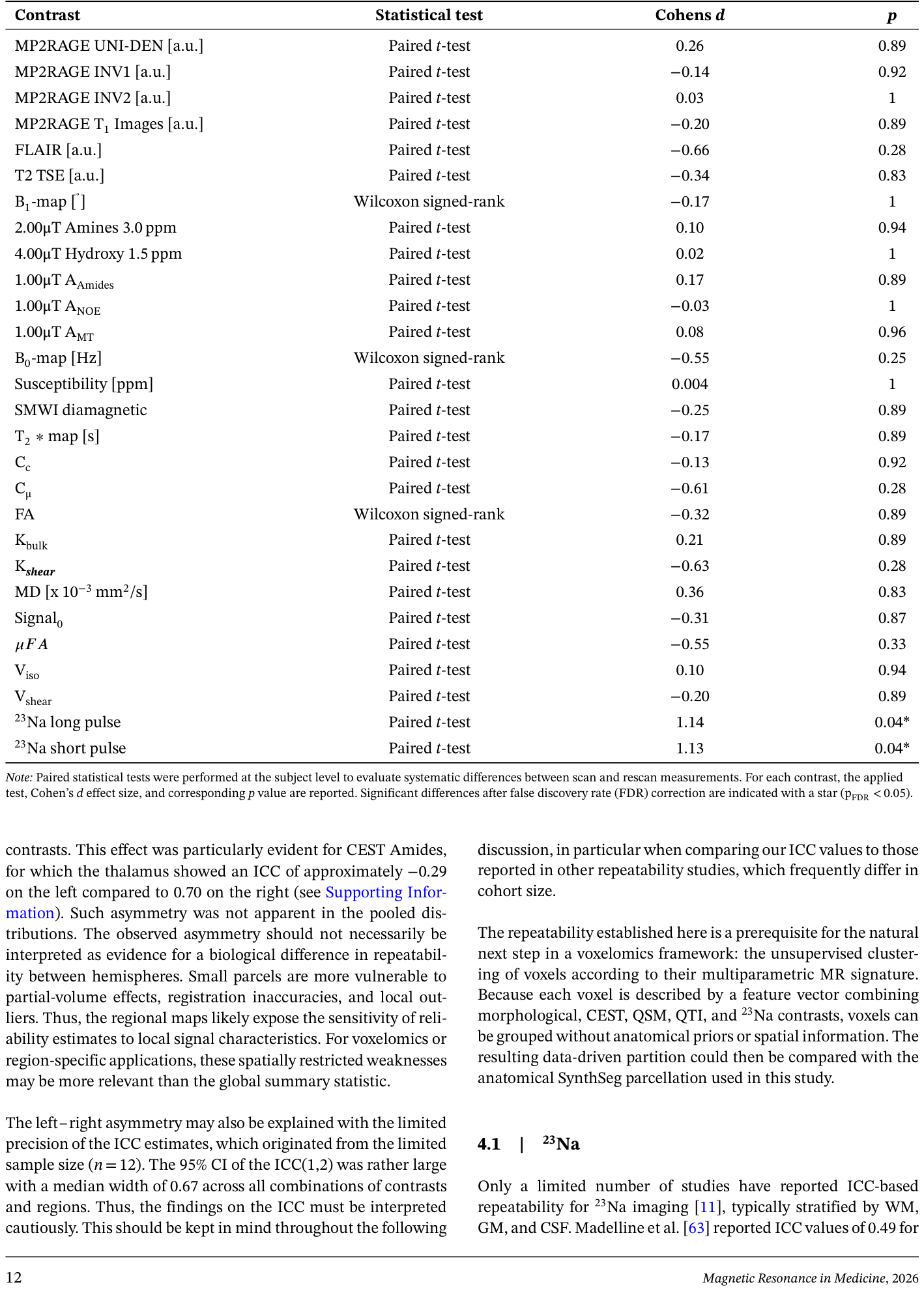
Table 2. TABLE 2 | Statistical assessment of systematic scan–rescan differences across imaging contrasts.解説: 各MRIコントラストにおける系統的なスキャン間差異を統計的に評価した結果を示す表です。適用された統計テスト、Cohenのd効果量、および対応するp値が報告されています。FDR補正後に有意差があったコントラストにはアスタリスクが付されています。
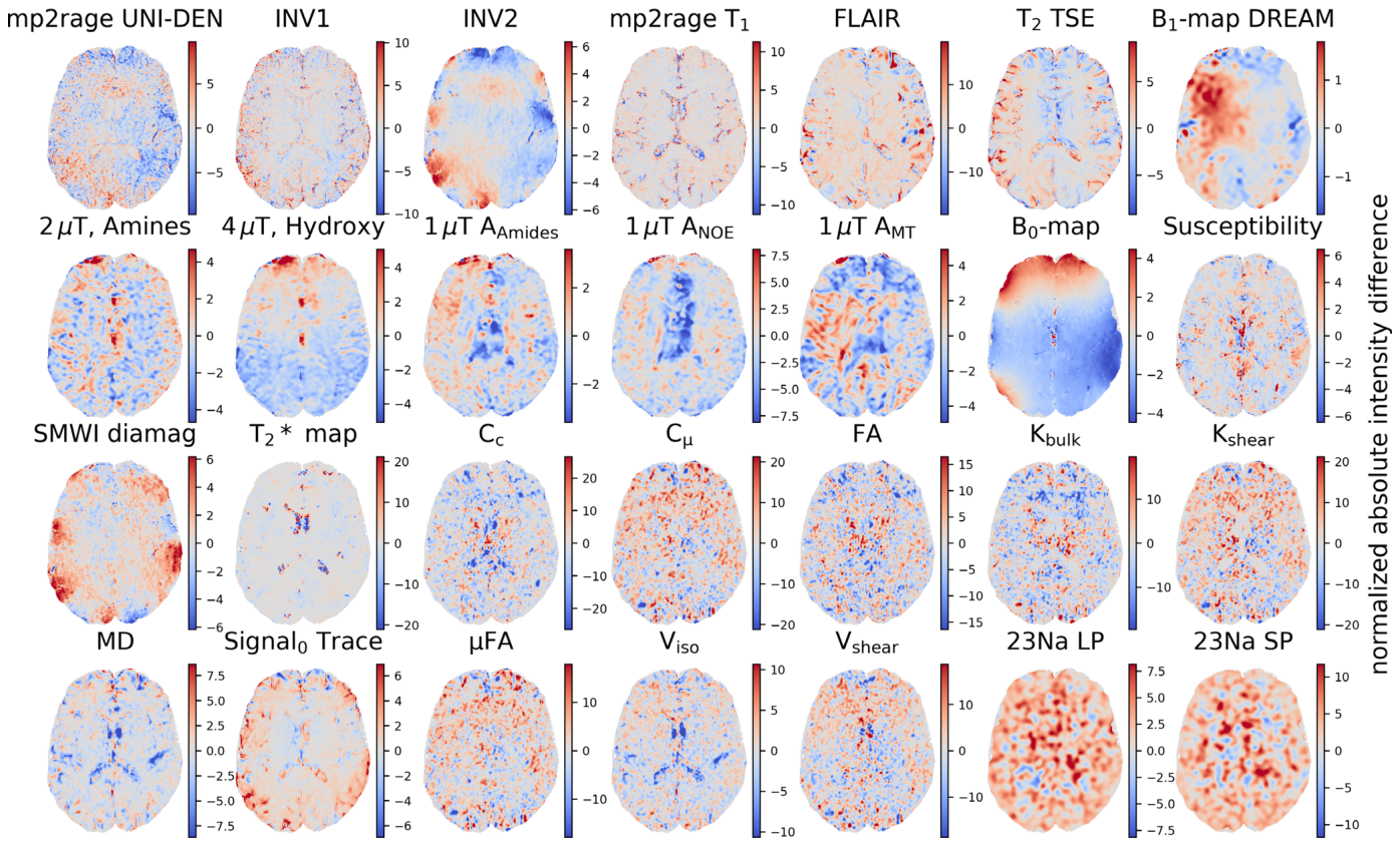
代表的な対象者におけるスキャン1とスキャン2の間のボクセルごとの相対的差分パーセンテージマップを
Figure 7. FIGURE 7 | Voxel-wise relative difference percentage maps with respect to the intensity range of Scan 2 for a representative subject. Difference maps (Scan1–Scan2), normalized to each contrast’s intensity range (% of full span), are shown for the same contrasts as in Figure 1, for a single representative subject. Because these maps reflect a single subject rather than a group average, localized effects such as the pronounced spatial dependency seen in the B0-map reflect scan-level specific field inhomogeneity rather than systematic group-level pattern.解説: 代表的な対象者について、スキャン1とスキャン2の間のボクセルごとの相対的差分パーセンテージマップです。差分マップは各コントラストの強度範囲に対して正規化されています。
コメントを残す