どうも、Beyond the Pixelです。拡散MRI(dMRI)は、脳の白質(神経線維が密集した部分)の微細な構造を非侵襲的に観察できる強力なツールです。dMRIは、水分子の拡散(広がり方)が、拡散をエンコードする強度(b値)や方向によってどのように変化するかを測定することで、組織の情報を得ます。この信号の変化を分析することで、私たちは白質を構成する神経線維の方向や密度などを推測することができます。
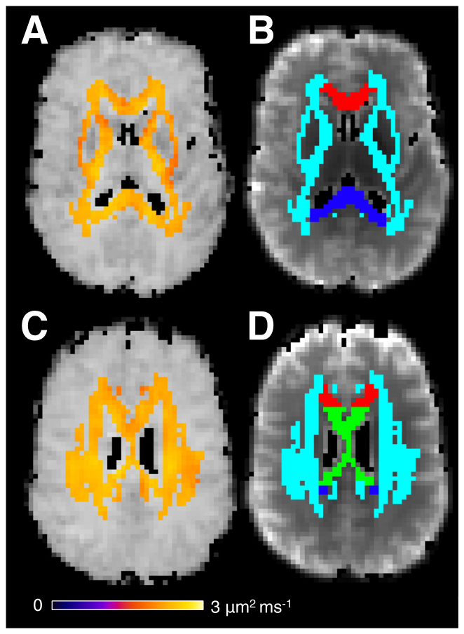
Figure 1. FIGURE 1 | White-matter regions of interest and independently measured intra-axonal diffusivity. In (A) and (C) the intra-axonal diffu- sivity (𝐷𝑎) estimated from triple diffusion encoding (TDE) MRI is shown for two axial image slices for a single subject. Panels (B) and (D) show the regions of interest used in the analysis: White matter (light blue), genu (red), body (green), and splenium (blue).解説: この図は、単一の対象者の2つの軸方向画像スライスにおける、三重拡散エンコーディング(TDE)MRIから推定された軸索内拡散係数(Da)と、解析に用いられた関心領域を示しています。(A)と(C)はDaを示し、(B)と(D)は白質(水色)、脳梁の膝(赤)、体部(緑)、膨大部(青)の関心領域を示しています。
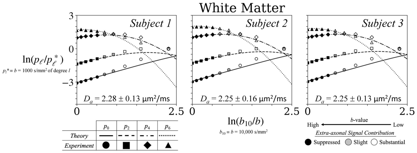
Figure 2. FIGURE 2 | Measured and predicted spherical harmonic powers in total white matter. White matter spherical harmonic power 𝑝𝑙of the dMRI signal plotted versus 𝑏for three subjects on log–log axes. The x-axis is ln(𝑏10∕𝑏) with 𝑏10 ≡10,000 s∕mm2, so 𝑏increases from right to left (1000 →10,000 s∕mm2). Harmonic powers are normalized within each degree by the 𝑏= 1000 s∕mm2 value, 𝑝∗解説: この図は、3名の対象者における全白質のdMRI信号の球面調和パワー(p_l)を、b値の関数として対数-対数軸上にプロットしたものです。y軸はln(p_l/p_l*)で、p_l*はl=1000 s/mm^2での調和パワーにより各次数内で正規化されています。x軸はln(b_10/b)で、b値は右から左に増加しています(1000 → 10000 s/mm^2)。実験データ(記号)とスティックモデルによる理論予測(破線)が比較されており、高b値(b ≳ 6000 s/mm^2)で最も強い一致が見られます。
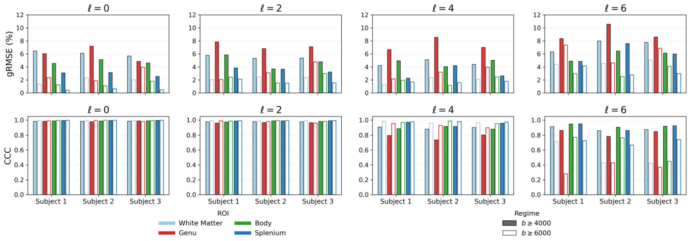
Figure 3. FIGURE 3 | Quantitative agreement between measured and stick-model-predicted harmonic-power curves. Subject-level agreement parameters: (top row) geometric root-mean-squared-error (gRMSE) to test “how wrong is the theory (in percent)?” and (bottom row) Lin’s concordance corre- lation coefficient (CCC) to answer “does the theory track the shape and level of the experimental curve?” Curves were fitted using the prespecified b ≥5000 s/mm2 range and subsequently evaluated without refitting over b ≥4000 and 6000 s/mm2. Agreement remained strong for l = 0, 2, and 4, and across evaluation thresholds. In contrast, l = 6 showed larger gRMSE and less stable CCC, particularly at the highest b-value threshold, supporting a more cautious interpretation of the highest harmonic degree.解説: この図は、測定された球面調和パワー曲線とスティックモデルの予測曲線との定量的な一致度を、対象者ごとの結果として示しています。上段は幾何平均二乗誤差(gRMSE)を、下段はリンのコンコーダンス相関係数(CCC)を示しています。曲線はb ≧ 5000 s/mm^2の範囲でフィッティングされ、その後b ≧ 4000 s/mm^2とb ≧ 6000 s/mm^2の範囲で再フィッティングせずに評価されました。l=0、2、4では評価閾値全体で強い一致が維持されていますが、l=6ではgRMSEが大きく、CCCの安定性が低いことが示されています。
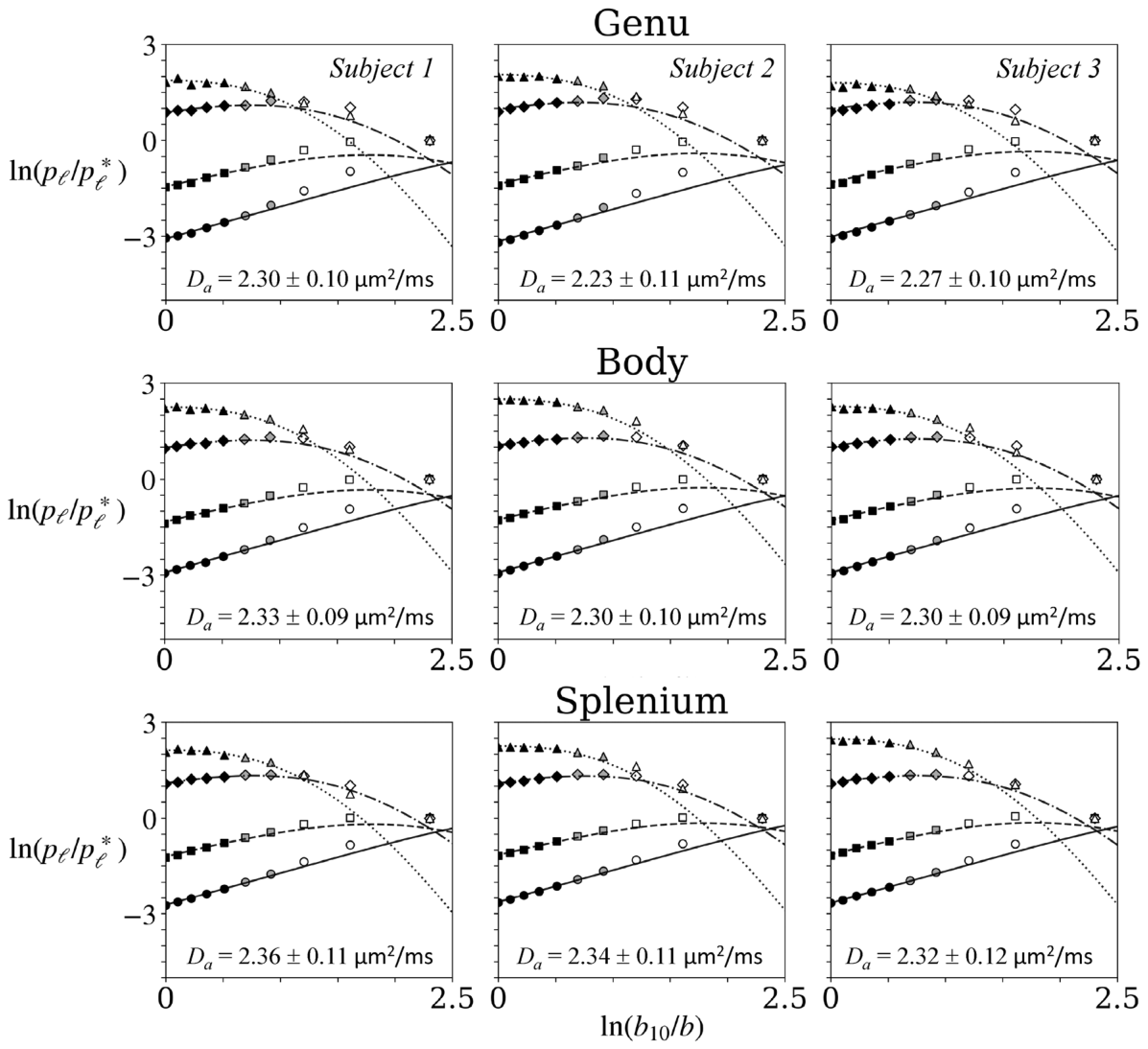
Figure 4. FIGURE 4 | Regional spherical harmonic powers and stick-model predictions within the corpus callosum. Here we illustrate the harmonic power for each degree (𝑝𝑙) of the spherical harmonic expansion of the dMRI signal as a function of the b-value for three subjects now within the genu, body, and splenium of the corpus callosum. The data are again presented on a log–log scale, and the symbols used are consistent with those in Figure 2. As observed throughout the entire white matter, there is a notable alignment with both theoretical predictions and experimental results for b ≥6000 s/mm2. Slightly greater variability is observed across all corpus callosum regions compared to the whole white matter, with the greatest variability in the genu for 𝑝6. Error bars are omitted since the standard errors of the mean are small in comparison to the size of the data symbols.解説: この図は、脳梁内の各関心領域(膝、体部、膨大部)におけるdMRI信号の球面調和パワー(p_l)とスティックモデルの予測を、3名の対象者について示しています。データは対数-対数スケールで提示され、記号はFigure 2と同様です。全白質と同様に、b ≳ 6000 s/mm^2で理論予測と実験結果が顕著に一致しています。
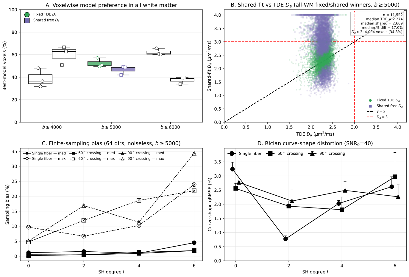
Figure 5. FIGURE 5 | 𝐷𝑎model comparison and Monte Carlo evaluation of finite-sampling and magnitude-noise effects. (A) Voxelwise AICc model pref- erence within total white matter for the two materially competitive formulations: Fixed independently measured TDE 𝐷𝑎and a single shared free 𝐷𝑎 across harmonic degrees. Boxes summarize subject-level percentages of all-white-matter voxels selecting each model across the three participants; cen- ter lines indicate medians, whiskers span the observed minimum and maximum, and points denote individual participants. The prespecified primary threshold, b ≥5000 s/mm2, is highlighted in color, whereas b ≥4000 and 6000 s/mm2 sensitivity analyses are shown in grayscale. Percentages are not renormalized after omission of the rarely selected degree-specific-𝐷𝑎model. (B) Voxelwise comparison of shared-fit and TDE-derived 𝐷𝑎for the primary b ≥5000 s/mm2 analysis. Purple circles indicate voxels favoring the fixed-TDE model and green squares indicate voxels favoring the shared- model. The black dashed line denotes identity, and red dashed reference lines indicate 𝐷𝑎= 3 μm2/ms. Voxels favoring the rarely selected degree-specific- model are omitted for visual clarity. (C) Monte Carlo estimates of finite angular-sampling error/bias for the experimental 64-direction acquisition in the absence of added noise, evaluated over b ≥5000 s/mm2. Marker shape denotes fiber geometry (single fiber, 60˚ crossing, or 90˚ crossing); solid curves show median sampling error/bias and dashed curves with overlaid crosses show maximum absolute bias. (D) Rician magnitude-noise-induced distortion of high- curve shape at SNR = 40, chosen to approximate the measured white-matter SNR. Points show median curve-shape gRMSE across orientations and upper error bars extend to the 95th percentile. Small horizontal offsets are applied only for visualization to reduce overlap. Together, these analyses show that fixed and shared 𝐷𝑎formulations are both supported voxelwise, whereas degree-specific 𝐷𝑎is rarely favored, and that finite sampling and magnitude noise increasingly affect higher-degree harmonic powers, particularly l = 6.解説: この図は、Daモデルの比較と、有限サンプリングおよびマグニチュードノイズの影響に関するモンテカルロ評価を示しています。(A)は全白質におけるボクセルごとのAICcモデル選好度を、(B)はフィットされた共有DaとTDE-Daのボクセルごとの比較を示しています。(C)はノイズなしで実験と同じ64方向取得における有限な角サンプリング誤差を、(D)はSNR=40でのライシアンマグニチュードノイズによる高b値曲線形状の歪みを示しています。

コメントを残す