光子計数型検出器を用いたヨウ素画像における散乱線の非線形な影響とSDNR低下の解明

10月 8, 2026 · 論文解説

🎧 この記事を音声で聴く（AI生成Podcast）

解説対象論文: Scatter-induced non-linear signal compression and SDNR loss in triple-energy photon-counting iodine imaging
Physics in Medicine and Biology｜被引用数: 0（2026年10月8日時点）

X線画像診断の最前線では、光子計数型検出器（PCD）が革新をもたらしています。この次世代技術は、X線光子をエネルギー別に識別し、診断画像から物質情報を詳細に分離することを可能にします。特に、造影剤として用いられるヨウ素の画像をより鮮明に、かつ正確に描出することで、血管の異常や病変の検出精度を向上させる潜在能力を秘めています。しかし、PCDを用いた高精細な画像診断においても、X線散乱線は画質を低下させる大きな課題として立ちはだかります。散乱線は、単に画像をぼやけさせるだけでなく、特にPCDの「三重エネルギー」画像処理において、ヨウ素の信号形成に予想外の非線形な影響を及ぼし、結果として画像の検出能（SDNR）を大幅に低下させることが示唆されています。本記事では、この重要な現象の背後にある物理学と、それがPCDを用いた造影画像にどのような影響を与えるのかを、最新の研究論文に基づき解説していきます。

研究サマリー（FINER & PICO）

Feasible実施可能性	既存の光子計数型検出器と標準的な実験室設定で実施可能であり、実用化に向けた基礎研究として実現可能です。
Ethical倫理面	本研究はファントムを用いた物理的評価であり、医療倫理委員会承認や対象者への影響に関する記述はありません。
Interesting面白さ	散乱線が三重エネルギー画像に非線形な信号圧縮を引き起こすという新規性の高い現象を明らかにしました。
Novel新規性	散乱線がエネルギービンごとに異なる影響を与え、三重エネルギー減算を通じてSDNRを非線形に低下させるメカニズムを定量的に示しました。
Relevant切実さ	光子計数型CTの臨床応用が進む中、造影剤を用いた血管画像診断の画質向上と最適化に直結する重要な知見を提供します。
Measurable測定可能性	ヨウ素の面積密度、散乱線分率、SDNRといった定量的な指標を用いて、散乱線の影響を詳細に評価しています。
Modifiable派生・改善	散乱線によるSDNR低下のメカニズム解明は、将来の散乱線補正技術や画像最適化戦略の開発に貢献します。
Structured文章構造	理論的導出、ファントムを用いた実験、およびシミュレーションを組み合わせた包括的かつ多角的なアプローチで研究が遂行されています。
PICO / PECO対象・介入・比較・結果	対象者(P): ヨウ素造影を受ける対象者。介入(I): 三重エネルギー光子計数型X線画像診断。比較(C): 散乱線の有無/レベル。結果(O): SDNR低下と非線形信号圧縮の定量化。

はじめに：次世代X線画像技術と散乱線の課題

どうも、Beyond the Pixelです。X線画像診断の分野では、光子計数型検出器（PCD）の登場により、大きな進化の波が押し寄せています。PCDは、X線光子を個別に検出し、そのエネルギーを測定できるため、従来の検出器では難しかった物質弁別（例えば、ヨウ素などの造影剤と軟部組織や骨を分離すること）を可能にします。これにより、造影剤を用いた血管画像診断において、病変の視認性を飛躍的に向上させる可能性を秘めています。すでに光子計数型CT（Computed Tomography）の臨床応用も進んでおり、この技術の重要性は日増しに高まっています。

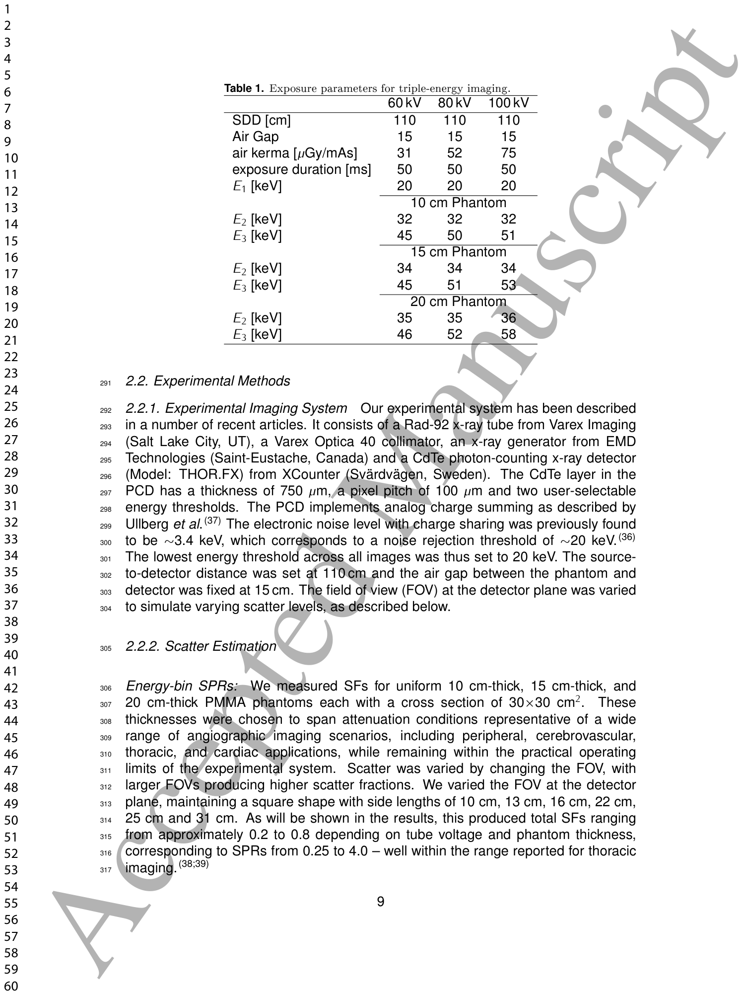
**Table 1.** Table 1. Exposure parameters for triple-energy imaging.解説: 三重エネルギー撮像の露出条件をまとめた表です。管電圧（60kV、80kV、100kV）ごとのSDD（光源から検出器までの距離）、エアギャップ、空気ケルマ、露出時間、および異なるファントム厚み（10cm、15cm、20cm）における各エネルギービン（E1、E2、E3）の閾値が示されています。

この研究では、PCDを用いた三重エネルギーX線画像における散乱線の影響、特にヨウ素の信号形成と画質指標であるSDNR（Signal-Difference-to-Noise Ratio、信号差対ノイズ比）への影響を定量的に明らかにすることを目指しています。

散乱線が引き起こす問題：信号の非線形な変化

PCDによる三重エネルギーX線画像では、3つの異なるエネルギー範囲のX線情報を取得し、これらを組み合わせることで軟部組織と骨の両方の信号を抑制し、ヨウ素固有の画像を生成できます。しかし、X線画像診断において常に課題となるのが散乱線です。散乱線とは、X線が対象者内部で散乱され、本来の経路から外れて検出器に到達するX線のことで、画像コントラストの低下や定量精度の劣化を引き起こします。特に、散乱線はエネルギー依存性を持つため、PCDで取得される各エネルギービン（特定のエネルギー範囲のX線がカウントされる区分）に異なる影響を与えます。このエネルギービンごとの散乱線の違いが、三重エネルギー減算処理（画像を合成する際の計算）を通じて非線形な信号の歪みを引き起こし、結果として画質を低下させる可能性があるのです。従来の研究では、散乱線が物質弁別の定量精度に与える影響は調べられてきましたが、三重エネルギー画像におけるヨウ素信号の形成や検出能（SDNR）への影響は、これまで体系的に検討されていませんでした。特に、三重エネルギー減算が非線形な演算であるため、散乱線がどのように影響を及ぼすかは自明ではありませんでした。

研究方法：理論、実験、そしてシミュレーション

本研究では、散乱線が三重エネルギー減算にどのように伝播し、ヨウ素信号差とSDNRに影響を与えるかを記述するための理論的枠組みを開発しました。この理論に基づき、エネルギービンごとの散乱線分率（SF）とヨウ素の面積密度との非線形な関係を考慮したヨウ素信号差、ノイズ、SDNRの解析式を導出しました。実験では、テルル化カドミウム（CdTe）ベースのPCDと画像品質評価用ファントムを使用しました。ファントムは、PMMA（アクリル樹脂）のスラブを重ねたもので、その中にアルミニウム製の挿入物、PMMAの空洞、PMMAの突起、そしてヨウ素溶液を満たしたウェルが含まれています。

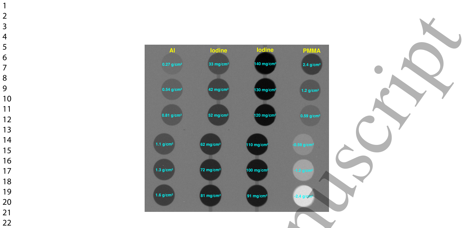
**Figure 1.** Figure 1. High-dose image of the phantom used for contrast and noise estimation. Left-most column: Al discs. Middle columns: iodine discs. Right-most column: PMMA discs.解説: コントラストとノイズ評価に使用されたファントムの高線量画像です。一番左の列はアルミニウムディスク、中央の列はヨウ素ディスク、一番右の列はPMMA（アクリル樹脂）ディスクを示しており、それぞれ異なる面積密度で構成されています。

これにより、ヨウ素の様々な面積密度（33〜140 mg/cm²）、散乱線分率（約0.2〜0.8）、管電圧（60〜100 kV）、ファントム厚（10〜20 cm）にわたってSDNRを評価しました。散乱線レベルは、X線照射野（FOV）を変えることで調整し、エアギャップ法を用いて定量化しました。実験データには、物理学に基づいた経験的モデルを当てはめ、その解釈を裏付けるために、チャージシェアリング（光子の相互作用で生じた電荷が複数のピクセルに広がる現象）やビームハーデニング（X線が物体を透過する際に低エネルギー成分が選択的に吸収され、平均エネルギーが高くなる現象）を含むシミュレーションも実施しました。本研究で使用されたPCDは、アナログチャージサミング（チャージシェアリングによるノイズを抑制する技術）を実装しており、ノイズ相関が低減されるため、理論的な仮定とも整合性が高いとされています。

主要な発見：散乱線による非線形信号圧縮とSDNR低下

この研究から、いくつかの重要な知見が得られました。まず、散乱線分率はエネルギービンによって異なり、最も低エネルギーのビンで最も高いSFを示すことがわかりました。

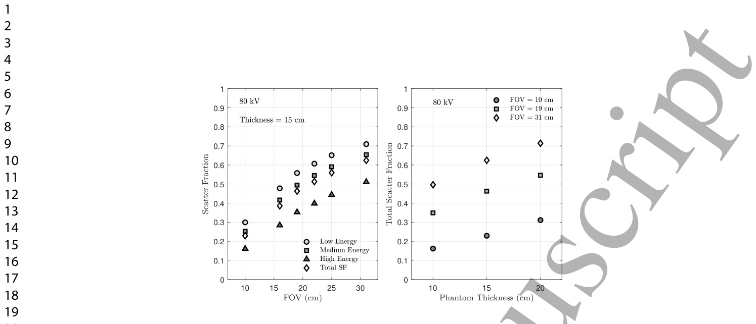
**Figure 2.** Figure 2. Scatter fraction trends across imaging conditions. (left) Energy-bin and total SF vs FOV (T = 15 cm, 80 kV). (Right) Total SF vs phantom thickness (80 kV, selected FOVs).解説: 様々な撮像条件における散乱線分率の傾向を示しています。左のグラフは、ファントム厚15cm、管電圧80kVの条件で、視野（FOV）のサイズに対する各エネルギービンおよび合計の散乱線分率（SF）の変化を表しています。右のグラフは、管電圧80kVで、ファントム厚に対する合計SFの変化を示しています。

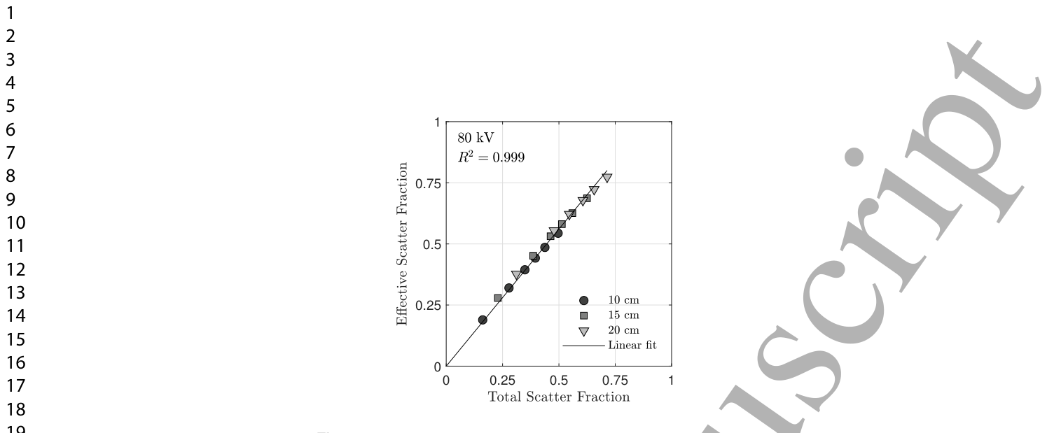
また、散乱線分率と合計散乱線分率の関係はほぼ線形であることが示されました。

**Figure 3.** Figure 3. Eective scatter fraction SFeff vs total scatter fraction SFtot for 80 kV. SFeff represents the weighted scatter fraction governing rst-order SDNR degradation in triple-energy imaging (Eqs. 21 – 22).解説: 80kVの条件における有効散乱線分率（SFeff）と合計散乱線分率（SFtot）の関係を示しています。SFeffは、三重エネルギー画像における一次SDNR劣化を支配する重み付けされた散乱線分率を意味します。グラフはほぼ線形（R² = 0.999）の関係を示しています。

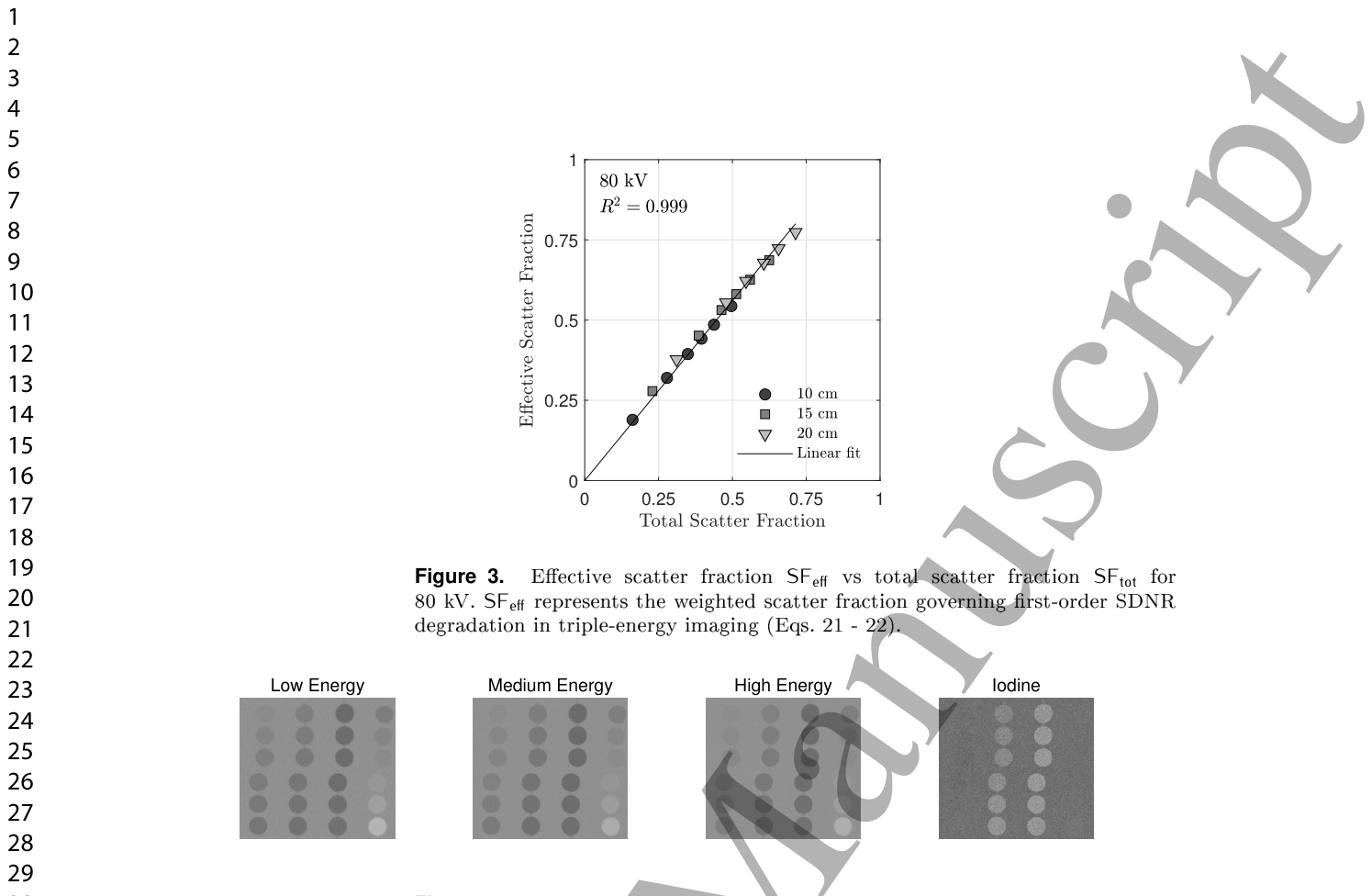
散乱線が増加すると、各エネルギービンにおけるヨウ素信号は、面積密度に対して非線形なカーブを描くようになりました。

**Figure 4.** Figure 4. Images from low-, medium-, and high-energy bins and their logarithmic combination to produce an iodine-speci c image. Results are shown for 60 kV, 15 cm thickness, and 19×19 cm2 FOV.解説: 低エネルギー、中エネルギー、高エネルギーの各ビンから取得された画像と、それらを対数的に組み合わせて生成されたヨウ素特異的画像を示しています。管電圧60kV、ファントム厚15cm、FOV19×19cm²の条件での結果です。⚠ 自動抽出画像の検証で一致を確認できませんでした。正確な内容は元論文のFigure 4をご参照ください。

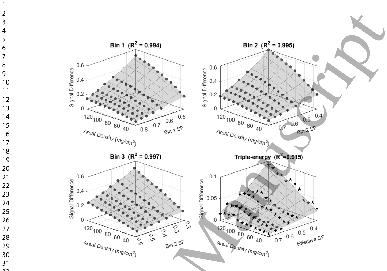
このエネルギービンごとの異なる反応が、三重エネルギー減算によって組み合わされると、三重エネルギー画像で著しい信号圧縮（信号の増加率が非線形に低下する現象）を引き起こすことが明らかになりました。

**Figure 5.** Figure 5. Signal dierences in log-transformed energy bin images and the triple energy images. Data are shown for an 80 kV tube voltage and a phantom thickness of 15 cm. Compression of the triple-energy signal emerges from diering curvature across energy bins, not from any single bin.解説: 対数変換されたエネルギービン画像と三重エネルギー画像における信号差を示しています。データは管電圧80kV、ファントム厚15cmの条件で取得されたものです。グラフは、ヨウ素面積密度と散乱線分率の関数として信号差がどのように変化するかを示しており、三重エネルギー信号の圧縮は個々のビンにおける曲率の違いから生じることを示唆しています。

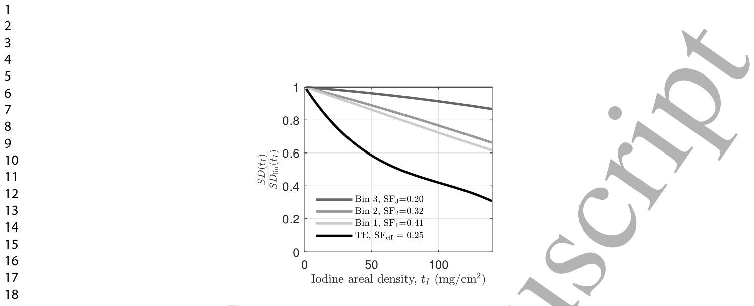
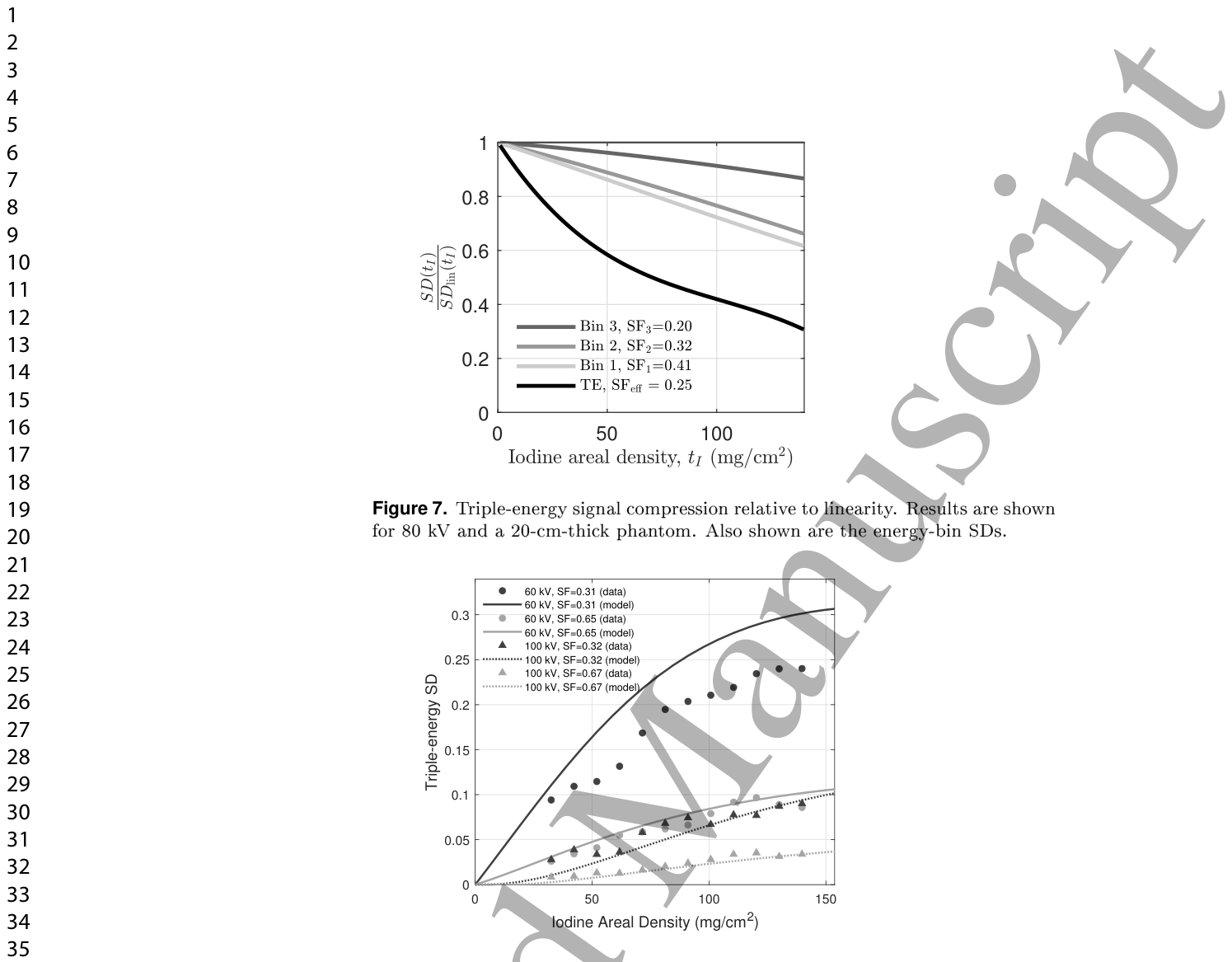
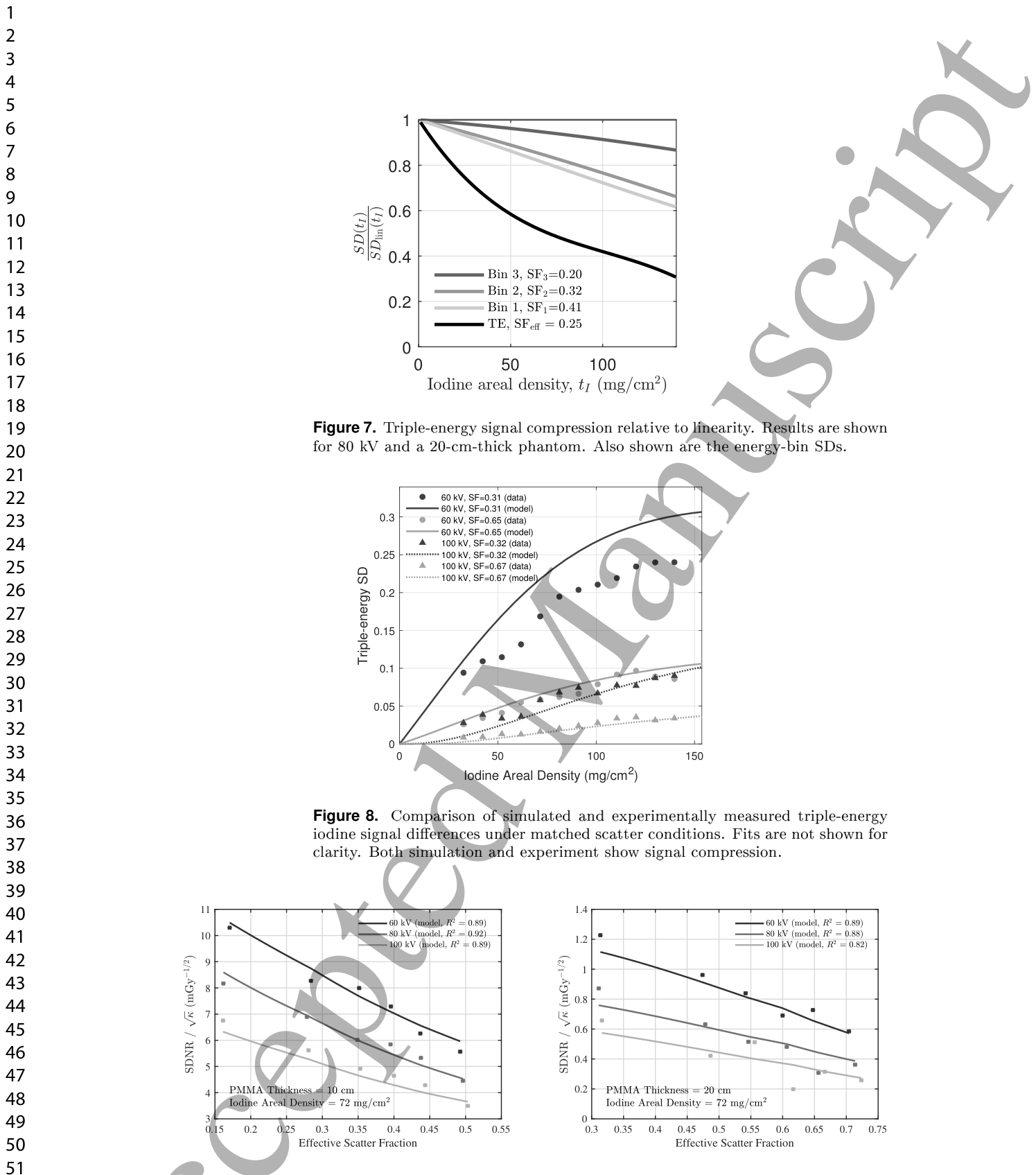
この信号圧縮は、個々のエネルギービンでの圧縮よりもはるかに強く、三重エネルギー画像合成の過程で散乱線とビームハーデニングの影響が複合的に作用していることを示唆しています。

**Figure 7.** Figure 7. Triple-energy signal compression relative to linearity. Results are shown for 80 kV and a 20-cm-thick phantom. Also shown are the energy-bin SDs.解説: 線形性に対する三重エネルギー信号圧縮の度合いを示しています。管電圧80kV、ファントム厚20cmの条件での結果です。個々のエネルギービン（Bin 1、Bin 2、Bin 3）の信号差（SD）も示されており、三重エネルギー画像の信号圧縮が個々のビンよりもはるかに強いことがわかります。

シミュレーションでも、この線形コントラスト損失と非線形圧縮の両方が再現され、この現象が画像チェーンに内在するものであることが確認されました。

**Figure 8.** Figure 8. Comparison of simulated and experimentally measured triple-energy iodine signal dierences under matched scatter conditions. Fits are not shown for clarity. Both simulation and experiment show signal compression.解説: シミュレーションと実験で測定された三重エネルギーヨウ素信号差の比較を示しています。散乱条件を一致させており、シミュレーションと実験の両方で信号圧縮が観察されています。

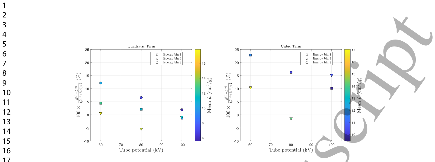
抽出された減衰係数は、異なる多項式の次数で一貫したエネルギー依存性を示しており、モデルの物理的整合性が確認されました。

**Figure 6.** Figure 6. Percent dierence between the linear estimate ˆµ(1) and the higher-order estimates ˆµ(n) for n = 2 and 3. Results are shown for a PMMA thickness of 20 cm. Marker shape denotes energy bin and marker color encodes the mean attenuation(ˆµ(1) + ˆµ(n))/2 (cm2/g).解説: 線形推定値ˆµ(1)と、2次（n=2）および3次（n=3）の高次推定値ˆµ(n)との間のパーセント差を示しています。結果はPMMA厚20cmの条件で示されており、マーカーの形状はエネルギービンを、マーカーの色は平均減衰量（ˆµ(1) + ˆµ(n))/2 (cm²/g)を表しています。

SDNRへの直接的な影響：性能低下は予想以上

SDNRの評価では、散乱線が増加するにつれてSDNRが単調に低下することが示されました。例えば、52 mg/cm²のヨウ素の場合、SFが約0.2でSDNRは約20%減少し、SFが約0.8では約70%も減少しました。

**Figure 9.** Figure 9. Kerma-normalized SDNR as a function of eective scatter fraction. Lines correspond to pro les through the tted 2D surface across the areal-density × scatter-fraction domain. Only a subset of areal-densities is shown.解説: 有効散乱線分率の関数としてのケルマ正規化SDNRを示しています。線は、面積密度と散乱線分率の領域全体にわたる当てはめられた2D表面からのプロファイルに対応しています。⚠ 自動抽出画像の検証で一致を確認できませんでした。正確な内容は元論文のFigure 9をご参照ください。

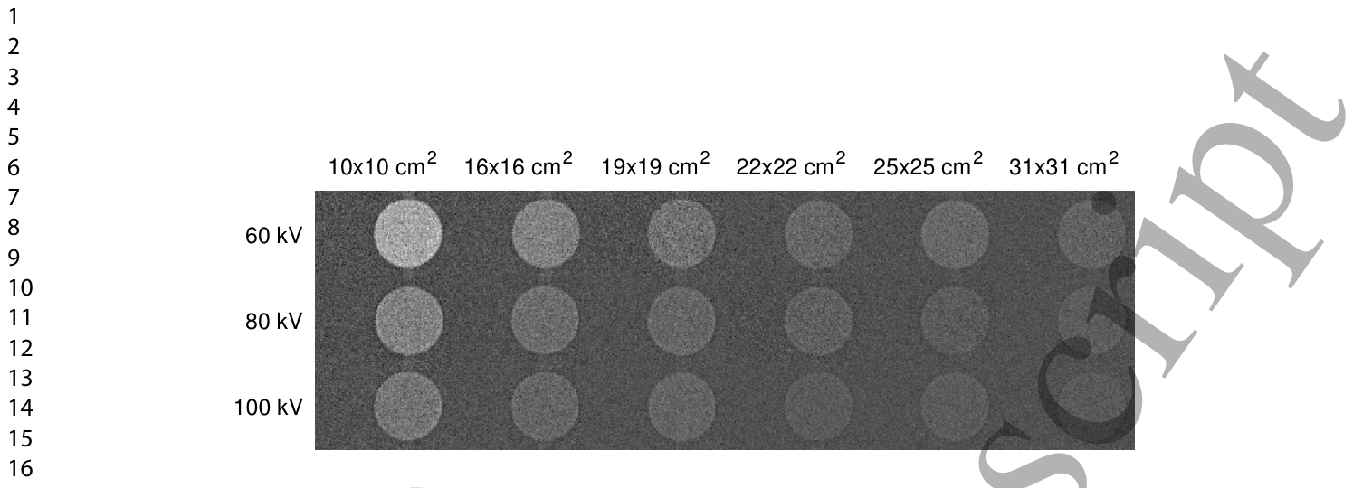
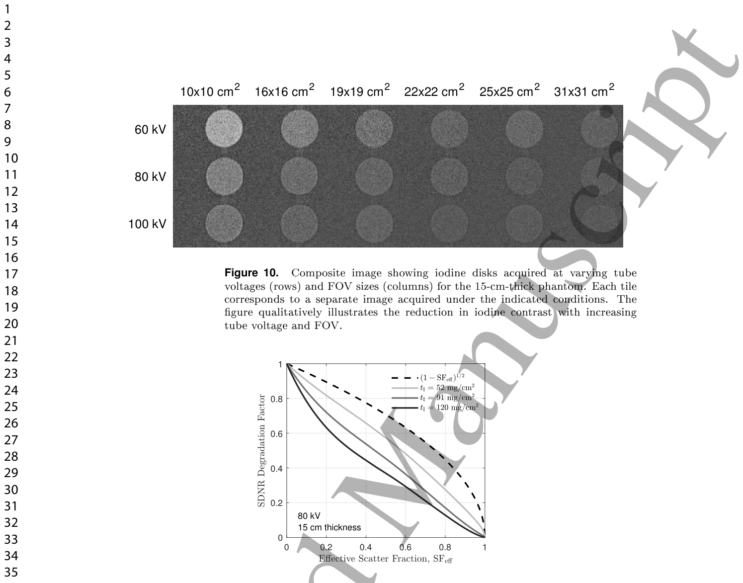
このSDNRの低下は、一次散乱スケーリング（散乱線によるコントラスト低下を単純な線形係数で近似する従来のモデル）から予想されるよりも顕著であることが判明しました。これは、散乱線がヨウ素の厚みが増すにつれて非線形信号圧縮を誘発し、SDNR損失を直接増幅するためです。また、ケルマ正規化SDNRは60kVで最も高かったですが、管電圧やFOVが変化するとヨウ素コントラストが低下することが視覚的にも示されました。

**Figure 10.** Figure 10. Composite image showing iodine disks acquired at varying tube voltages (rows) and FOV sizes (columns) for the 15-cm-thick phantom. Each tile corresponds to a separate image acquired under the indicated conditions. The gure qualitatively illustrates the reduction in iodine contrast with increasing tube voltage and FOV.解説: 15cm厚のファントムに対して、様々な管電圧（行）と視野（FOV）サイズ（列）で取得されたヨウ素ディスクの複合画像です。各タイルは、指定された条件下で取得された個別の画像に対応しており、管電圧およびFOVの増加に伴うヨウ素コントラストの低下を視覚的に示しています。

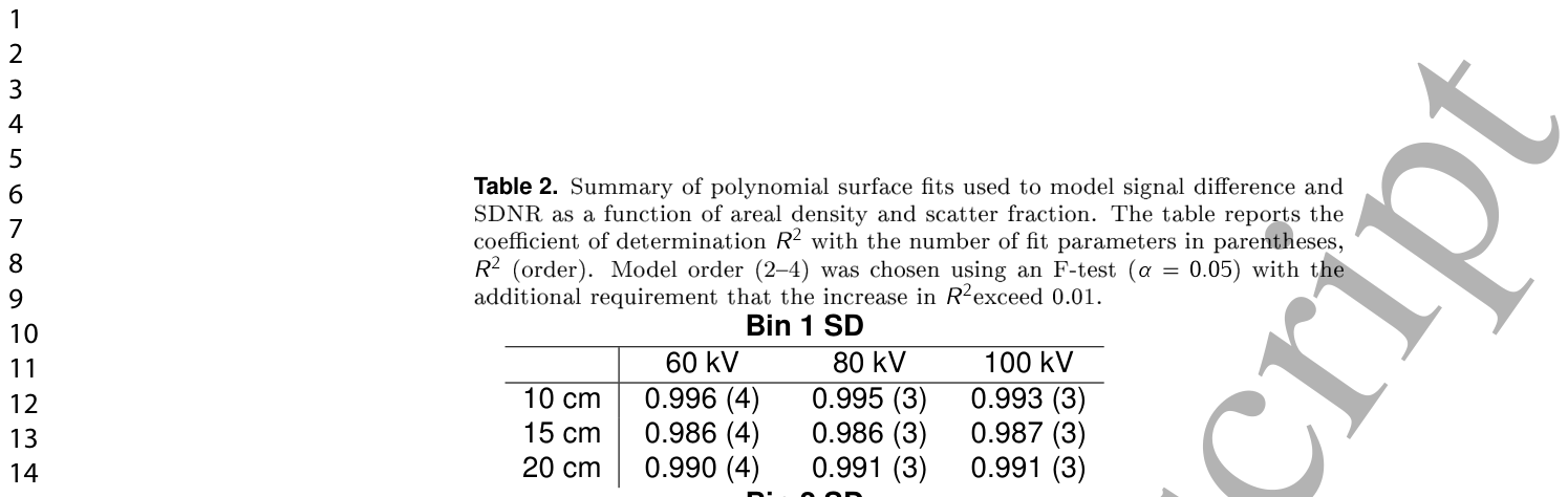
この研究で開発されたSDNRモデルは、測定データと高い一致度を示し、散乱線とノイズに関するモデルの依存性がSDNR低下の主要な挙動を捉えていることが確認されました。

**Table 2.** Table 2. Summary of polynomial surface ts used to model signal dierence and SDNR as a function of areal density and scatter fraction. The table reports the coe cient of determination R2 with the number of t parameters in parentheses, R2 (order). Model order (24) was chosen using an F-test (α = 0.05) with the additional requirement that the increase in R2exceed 0.01.解説: 面積密度と散乱線分率の関数として、信号差とSDNRをモデル化するために使用された多項式曲面近似の要約表です。決定係数R²（モデルの次数）が示されており、モデルの次数はF検定（α=0.05）とR²の増加が0.01を超えるという追加要件に基づいて選択されました。

研究の意義と今後の展望

本研究は、エネルギービンに依存する散乱線が、三重エネルギー画像における非線形信号圧縮を引き起こし、ヨウ素厚の増加に伴うSDNR損失を直接増幅するという新たな知見を提供します。この挙動は、三重エネルギー減算の構造に起因するため、従来の一次散乱スケーリングでは性能低下を過小評価してしまう可能性があります。この研究で確立された理論的および実験的解析の枠組みは、光子計数型血管造影画像における散乱線による画像劣化を軽減するための戦略（散乱線除去や散乱線補正技術など）を評価するための物理学的基盤となります。今後は、本研究で得られた知見を基に、より効果的な散乱線補正アルゴリズムの開発や、PCDを用いた次世代X線画像診断システムの最適化が進むことが期待されます。

補足図表

Figure 11

用語集

光子計数型検出器 (PCD): X線光子を個別に検出し、そのエネルギーを測定できる次世代のX線検出器です。
物質弁別: 異なるX線エネルギー情報を用いて、画像中の物質（軟部組織、骨、造影剤など）を分離する技術です。
散乱線: X線が物体を通過する際に散乱され、本来の経路から外れて検出器に到達するX線。画像コントラストを低下させます。
SDNR (Signal-Difference-to-Noise Ratio): 信号差対ノイズ比。画像中の関心領域と背景領域の信号差をノイズで割った値で、信号の検出能を示す指標です。
散乱線分率 (SF): 検出器に到達するX線のうち、散乱線が占める割合です。
三重エネルギーX線画像: 3つの異なるエネルギー範囲のX線情報を用いて画像を生成する技術。複数の物質を同時に分離・抑制できます。
信号圧縮: 信号の増加率が非線形に低下する現象で、特に高濃度領域で信号が飽和し、コントラストが失われるように見えます。
面積密度: 単位面積あたりの物質の質量。画像診断では、X線ビームが通過する物質の厚みと密度の積で表されます。
一次散乱スケーリング: 散乱線が画像コントラストに与える影響を、信号に一定の係数（1-SF）を乗じることで線形に近似するモデルです。
チャージシェアリング: X線光子が検出器内で相互作用した際に生じた電荷が、隣接する複数のピクセルに広がる現象です。
ビームハーデニング: X線が物体を透過する際に、低エネルギー成分が選択的に吸収され、X線スペクトルの平均エネルギーが高くなる現象です。