どうも、Beyond the Pixelです。分子放射線療法(MRT)は、転移性去勢抵抗性前立腺がん(mCRPC)に対する[177Lu]Lu-PSMA-617療法のように、特定の疾患に対する有効な治療法として確立されつつあります。この治療法では、腫瘍に高い吸収線量を送りながら、腎臓などのリスク臓器への不必要な放射線被曝を最小限に抑えることが不可欠です。そのため、対象者ごとの堅牢な線量評価は、治療計画の最適化において極めて重要な役割を果たします。従来の線量評価では、複数の画像撮影時点でのデータが必要となり、これらは対象者の負担増加、被曝量の増大、および臨床リソースへの大きな負荷を伴います。これらの課題に対処するため、一点撮像(STP)線量評価が実用的な代替手段として提案されています。STP線量評価は、単一の画像取得から時間積分活性係数(TIAC)を推定することを目的としており、データ収集を大幅に簡素化しながらも許容可能な線量評価性能を維持します。しかし、これまでの研究では、STP線量評価の精度が、集団レベルでの評価では許容範囲内であっても、個々の対象者レベルでは大きなばらつきが生じる可能性が指摘されていました。このことは、単一の画像取得タイミングの選択が、臨床的に信頼できるSTP線量評価の実現において極めて重要であることを示しています。
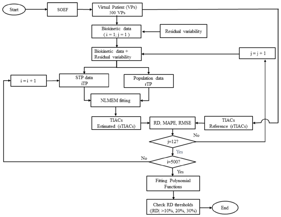
Figure 1. Fig. 1 Study workflow. The SOEF model (Eq. 1) was used to generate 500 virtual patients (VPs), and reference TIACs (rTIACs) were calculated analytically. Biokinetic data were simulated with added intra-individual variability. Simulated biokinetic data at twelve investigational time points (iTPs) were evaluated for STP dosimetry, whereas simulated biokinetic data at five reference time points (rTPs) [1] were used as the population data for NLMEM. Pop ulation biokinetic data at the rTPs were simultaneously fitted with the STP biokinetic data at each iTP data using NLMEM. STP-estimated TIACs (sTIACs) were compared with rTIACs using RD, RMSE, and MAPE. Fitting of RMSE-time and MAPE-time trends identified the optimal STP imaging time point. Absolute RDs exceeding 10%, 20%, and 30% were used for patient-level analysis. i = virtual patient index; j = investigational time point解説: 本研究のVP-NLMEMワークフローを示しています。SOEFモデルを用いて500の仮想対象者を生成し、参照TIACを解析的に計算します。その後、仮想対象者ごとに生体動態データがシミュレートされ、測定誤差が加えられます。STP線量評価のために12の調査時点(iTPs)が評価され、5つの参照時点(rTPs)が生体動態データとして使用されます。これらのデータはNLMEMを用いて同時にフィッティングされ、STP推定TIAC(sTIACs)が計算されます。sTIACsはRD、RMSE、MAPEを用いてrTIACsと比較され、RMSE-時間およびMAPE-時間のトレンドのフィッティングにより最適なSTP画像取得時点が特定されます。個人レベルの分析のために、絶対RDが10%、20%、30%を超える対象者が特定されます。
最適化された一点撮像タイミング:注目の結果
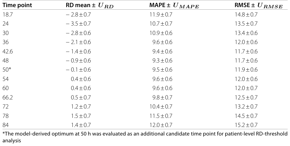
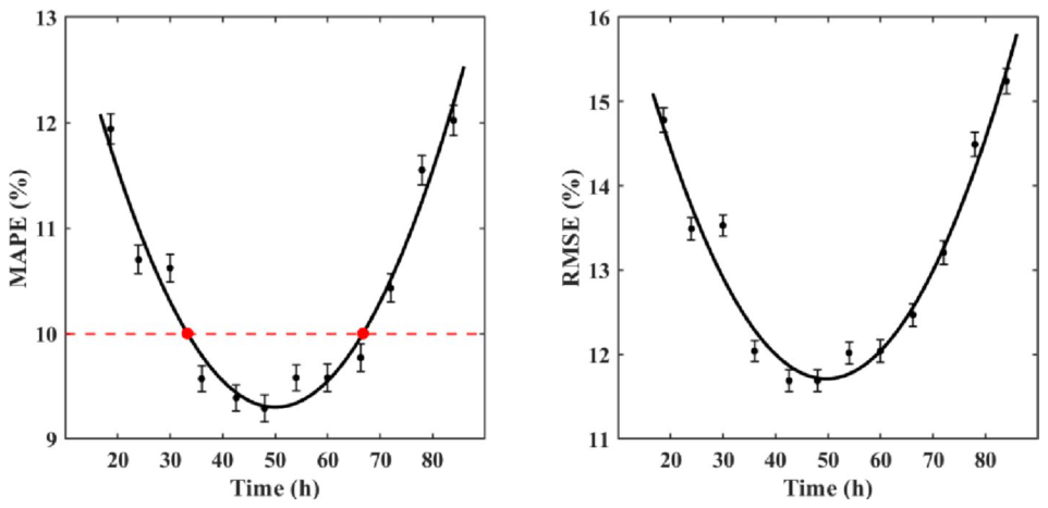
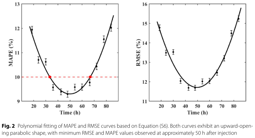
本研究におけるSTPシミュレーションの結果は、 investigated time points(iTPs)全体で、最も低いMAPEとRMSEの値が48時間でそれぞれ9.3% ± 0.6%と11.7% ± 0.6%であったことを示しました。これよりも早い時点ではMAPEとRMSEの値は一般的に高く、54時間以降で再び増加しました。多項式モデルによるMAPE-時間およびRMSE-時間のトレンドのフィッティングは、両曲線が注入後約50時間で顕著な最小値を示すことを明らかにしました。これは、調査された画像取得時点の中で、最も低い集団レベルの誤差指標が48時間で観察されたことと一致しています。さらに、多項式モデリングは、約50時間(約33~67時間)を中心とした最適値の存在を予測しました。
Figure 2. Fig. 2 Polynomial fitting of MAPE and RMSE curves based on Equation (S6). Both curves exhibit an upward-open ing parabolic shape, with minimum RMSE and MAPE values observed at approximately 50 h after injection解説: 多項式モデル(Equation (S6)に基づく)を用いたMAPEおよびRMSE曲線のフィッティング結果を示しています。両曲線は上に開く放物線形状を示し、RMSEとMAPEの最小値は注入後約50時間で観察されました。
Figure 3. Figure 3 shows a comparison between time-activity curves from reference and STP, consisting of (a) the minimum (VP 102) RD, (b) the median (VP 483), and (c) the maxi mum RD (VP 150). The comparison demonstrates that for patients with minimum RD, the STP-predicted kinetics closely match the reference kinetics. The median case shows a moderate level, while patients with higher RD exhibit noticeable discrepancies, par ticularly at early and late time points.解説: 選択された仮想対象者(VPs)のモデル推定時系列活性曲線(TACs)と参照TACsの比較を示しています。(a)最小RD(VP 102)、(b)中央値RD(VP 483)、(c)最大RD(VP 150)の対象者について比較が行われています。最小RDの対象者ではSTP予測の動態が参照動態と密接に一致する一方、最大RDの対象者では特に早期および後期において顕著な不一致が見られます。⚠ 自動抽出画像の検証で一致を確認できませんでした。正確な内容は元論文のFigure 3をご参照ください。
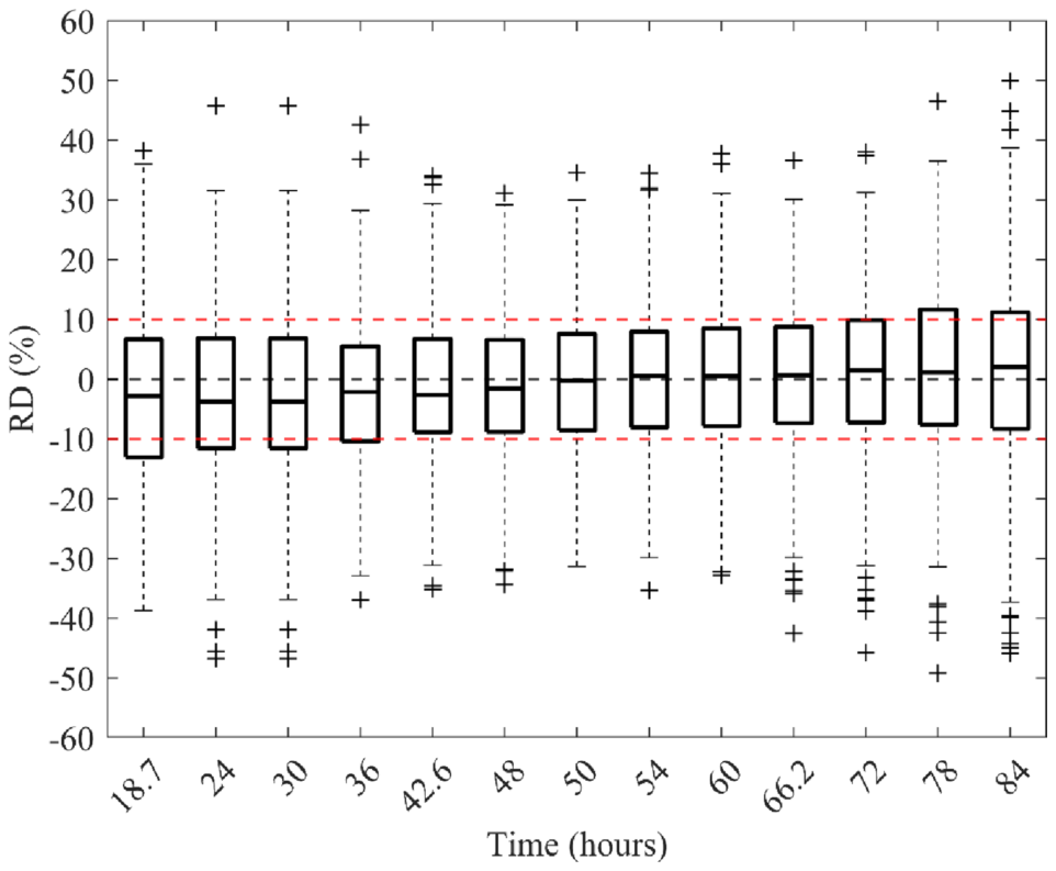
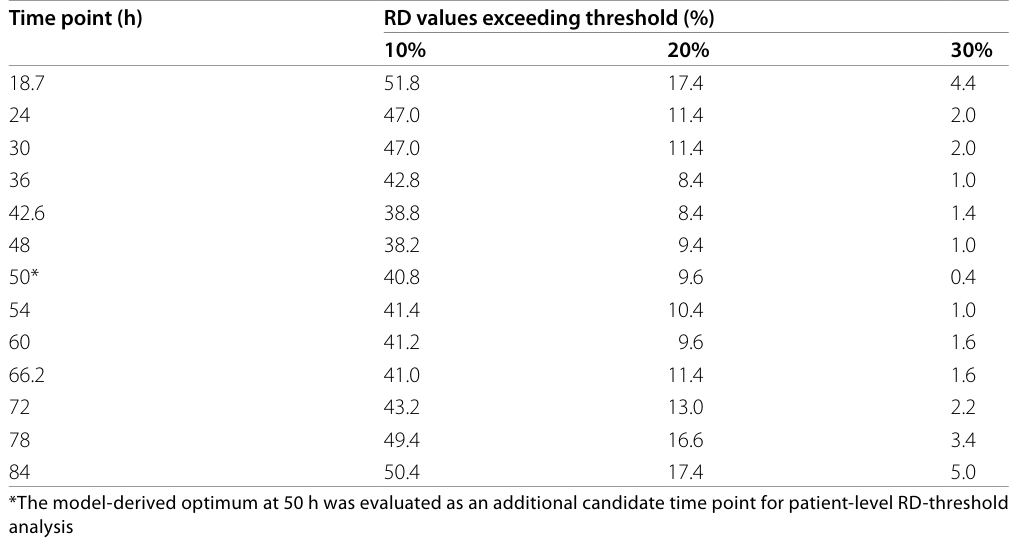
Figure 4. Fig. 4 Distribution of relative deviations (RD) across 12 investigated imaging time points (18.7–84 h post-injection) and for the additional model-derived 50 h time point. The 50 h time point was obtained from polynomial fitting and subsequently evaluated by an additional VP-NLMEM simulation to assess the individual-level RD distribution. Boxplots display the median RD and statistical outliers (values beyond 1.5×IQR). Notably fewer outliers were ob served at 50 h after injection, indicating reduced interpatient variability at this time point解説: 注入後12の調査時点(18.7~84時間)とモデルによって導き出された最適な50時間の追加評価時点における相対偏差(RD)の分布を示しています。箱ひげ図はRDの中央値と統計的な外れ値(IQRの1.5倍を超える値)を示しており、注入後50時間で外れ値が著しく少ないことが観察され、この時点での対象者間のばらつきが低いことを示唆しています。

コメントを残す